Introduction

The problem of phase change (Stefan problem) around a cylindrical source occurs in many engineering designs: oil/gas production/injection wells in permafrost areas, underground pipelines, steam production boreholes, melting of metals and storage of nuclear waste. In the cylindrical coordinates, an exact solution of the Stefan problem in the infinite domain exists only for two cases: subcooled liquid, which freezes while the solidified region remains at the fusion temperature; and a line source, which extracts energy at some constant rate per unit length (Carslaw & Jaeger 1959). Heat balance integral solutions were applied to the problem of finite superheat, when the initial temperature of the medium is lower than the fusion temperature (Tien & Churchill 1965; Sparrow et al. 1978; Lunardini 1988). Different numerical methods were used to solve the heat valance integral equations, but the results were essentially the same (Lunardini 1988). A coordinate transformation method reduced the problem with a variable phase change, such as a cylinder, to one with a constant phase change area (Lin 1971). An interesting effective thermal diffusivity concept was introduced (Churchill & Gupta 1977). It was assumed that the actual thermal diffusivity could be replaced by the effective thermal diffusivity, which includes the latent heat. The accuracy of these two methods is limited to certain ranges of dimensionless parameters (Lunardini 1988).

When wells are drilled through permafrost, the natural temperature field of the formations in the vicinity of the borehole is disturbed and the frozen rocks thaw for some distance from the borehole axis (e.g., Romanovsky et al. 2007; Eppelbaum et al. 2014). Making geothermal measurements to determine the static temperature of the formation and the permafrost thickness must be postponed for some period after completion of the drilling. This is the so-called restoration time. A lengthy restoration period of up to 10 years or more is required to determine the temperature and thickness of permafrost with sufficient accuracy (Lachenbruch & Brewer 1959; Melnikov et al. 1973; Shiu & Beggs 1980; Judge et al. 1981; Taylor et al. 1982; Clow 2014; Eppelbaum et al. 2014). The duration of the refreezing of the layer thawed during drilling is very dependent on the natural temperature of the formation; therefore, the rocks at the bottom of the permafrost refreeze very slowly (e.g., Dobinski 2011). The position of the interface of the thawing–freezing transition can be determined with resistivity and sonic logs. For example, the transition from higher resistivity and velocity readings to lower values can be considered as the position of the thawing radius. In our recent paper, we suggested a method to estimate how long it takes for formations thawed by drilling to refreeze (Kutasov & Eppelbaum 2017a, b). The method requires just three temperature logs taken after the freezeback is completed. Earlier we conducted numerical modelling and found that the dimensionless time of refreezing can be expressed as a function of two dimensionless parameters: the dimensionless radius of thawing and the dimensionless latent heat density (Kutasov 1999, 2006). Kutasov et al. (1977) proposed an effective approach for solving the problem of phase change (Stefan problem) around a cylindrical source of heat. It was shown that a known solution for a planar system can be utilized to obtain an approximate solution of the Stefan problem for a cylindrical source of heat with a constant temperature. Later (Kutasov 1998), we used an adjusted heating time concept (Kutasov 1987, 1999) to determine the position of a thawing temperature isotherm in the problem without the ice–water transition. The results of numerical solutions presented in Taylor (1978) were used to verify the results of our calculations.

It was shown that for a cylindrical system the position of the phase interface in the Stefan problem can be approximated through two functions. One function (r_m) determines the position of the melting-temperature isotherm in the problem without phase transitions, and the second function Ψ does not depend on the time (Kutasov et al. 1977; Kutasov 1998, 2006; Eppelbaum et al. 2014). Recently, Wang et al. (2017) reported an interesting study in which they developed a coupled thermal model of the wellbore–permafrost system. It considered the latent heat of fusion, water migration and the change in thermal parameters. In this study, work done by Ramey (1962) and the temperature prediction model for incompressible fluids developed by Wu & Pruess (1990) and Hasan and Kabir (1994) were used to describe heat transfer in the borehole-formation system. Numerical solutions of moisture transfer problems for frozen soil were based on the equations given by Harlan (1973). For numerical simulations, Wang et al. (2017) selected a simulation well: well depth is 3100 m and thickness of permafrost is 750 m. The suggested coupled thermal model of the wellbore in permafrost regions allowed for the estimation of the volume of thawed permafrost (and the corresponding radius of thawing) and radial temperature of formations. It was also shown that the use of low thermal conductivity cements significantly reduces the volume of thawed permafrost. The most important result of the study by Wang et al. (2017) is the following: very low rate of water migration (only 4.72 × 10⁻⁵ m³/s) (see the parameters for a simulated well, Table 1 in Wang et al. 2017). As a result, the heat transferred with the water migration is negligible compared with the heat caused by heat conduction. The simulation results (radius of thawing) can be validated against data obtained by geophysical logging (see also end of the “Time of the complete freezeback” section) and by temperature logs taken during shut-in (the degree of thermal disturbance caused by drilling).

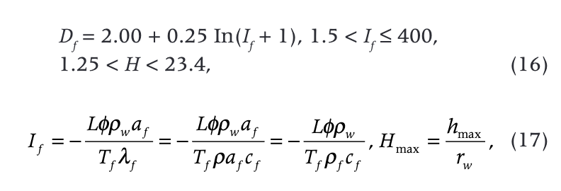
The objective of this study is to estimate the dynamics of the unfrozen zone (radius of thawing during drilling and shut-in periods). To demonstrate the applicability of the suggested equations in estimating the formation temperature, the radius of thawing and the time of complete freezeback in a field case are presented.

The drilling period

The results of field and analytical investigations have shown that in many cases the effective temperature (T_w) of the circulating fluid (mud) at a given depth can be assumed constant during drilling or production (Lachenbruch & Brewer 1959; Jaeger 1961; Edwardson et al. 1962; Ramey 1962; Kutasov et al. 1966; Raymond 1969). Here we should note that even for a continuous mud circulation process the wellbore temperature is dependent on the current well depth and other factors. The term “effective fluid temperature” is used to describe the temperature disturbance of formations while drilling. We should note that the effective temperature T_w takes into account the changes in heat transfer during all period of mud circulation on the given depth. The good agreement between calculated values of transient (shut-in) temperatures and the results of temperature surveys in numerous wellbores in permafrost regions confirms this assumption (Kutasov 1999; Kutasov & Eppelbaum 2003). Because of its low permeability, water migration is usually neglected in permafrost studies. Recent numerical modelling was used to confirm this assumption (Wang et al. 2017).

Lachenbruch & Brewer (1959) have shown that the wellbore shut-in temperature mainly depends on the amount of thermal energy transferred to (or from) formations. Therefore, for every depth a value of T_w can be estimated from shut-in temperature logs. Drawing from Kutasov’s earlier work (1977, 1998, 2006), we can write that

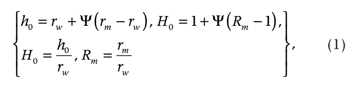
where r_w is the radius of the well and h₀ is the radius of thawing. The function r_m determines the position of the melting-temperature isotherm in the problem with phase transition. The function Ψ shows to what extent the melting process affects the position of the melting-temperature isotherm and does not depend on time. From physical considerations, it follows that 0 < Ψ < 1. The function r_m is known, but is expressed through a complex integral. By introducing an adjusted dimensionless heating time (t_D*), we have found (Kutasov 1987) that the exponential integral (a tabulated function) can be used to approximate the function T_D = T(r_D, t_D):

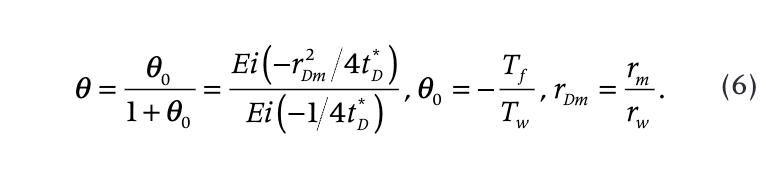
where r is the cylindrical coordinate, r_D is the dimensionless radial distance, Ei(x) is the exponential integral, T_w is the temperature at the wall of the borehole, T_m is the temperature of melting, T_f is the initial temperature, T(r, t) is the radial temperature, T(r_D, t_D) is the dimensionless radial temperature, t_D is the dimensionless time and a₁ is the thermal diffusivity of the frozen formation.

The correlation coefficient G(t_D) varies in the narrow limits: G(0) = 2 and G(∞) = 1. From Eqn. 2 (assuming that T = T_m) we can determine the position of the melting-temperature isotherm. In our case, the melting temperature (for pure ice) is 0°C, and the following equation can be used to determine r_m

As can be seen from Table 1, Eqn. 6 approximates the position of 0°C isotherm with good accuracy.

Analysis of physical characteristics indicates that at the very small times the solutions for cylindrical systems approach those for plane systems. For this reason, we assumed that the function Ψ can be determined from the known solution for the plane Stefan problem (Carslaw & Jaeger 1959). In a plane system, the position of the solid–melted interface is

Here, subscripts ₁ and ₂ correspond to the frozen and thawed zones, respectively, l is the thermal conductivity, c is the specific heat, T_s is the surface temperature, r is the density, L is the latent heat per unit of mass, w is the ice mass content per unit of volume, Φ is the probability integral and Φ* = 1 – Φ.

Introducing the dimensionless parameters, we obtain

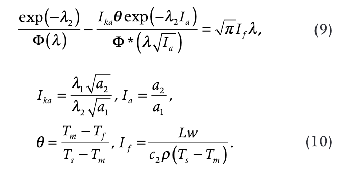
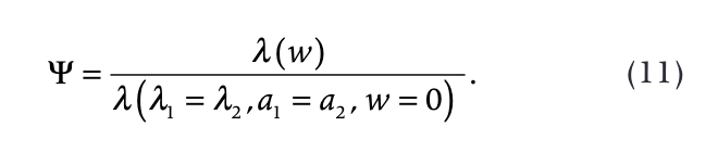
As we can see (Eqn. 7), the depth of thawing X is a product of two functions and the function l does not depend on time. The changes of thermal properties are due to thawing, and therefore, by using our assumption, we obtain from Eqn. 8 that

The results of a numerical solution (Taylor 1978) and results of calculations (after Eqns. 1–10) were compared (Kutasov 2006). It was found that both approximate solutions are in satisfactory agreement.

Shut-in period

After the cessation of the drilling process, the radius of thawing and the radius of thermal influence will increase for a definite period of time Δt₀ at the expense of the heat accumulated in the thawed zone. Correspondingly, the increase of the radius of thawing will be Δh₀. We suggested an empirical relationship to estimate the parameter Δt₀ (Kutasov 1999: 181). Hydrodynamical modelling (Kutasov 1999) has shown that the maximum value of the thawing radius can be given by

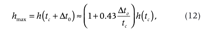
where t_c is the drilling mud circulation time at a given depth.

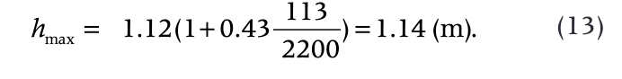
As an example, the results of one iteration of the hydrodynamic modelling are presented in Fig. 1. The input parameters are the time of heating disturbance t_c = 2200 hr, the temperature of drilling mud is T_m = 8°C, the temperature of the formation is T_f = −2°C, the well radius is r_w = 0.1 m, thermal diffusivity and thermal conductivity of the thawed formation is a_t = 0.0030 m²/h and l_t = 2.0 kcal/(h·m·°C) and the thermal conductivity of the permafrost (frozen area) is l_f = 2.5 kcal/(h·m·°C).

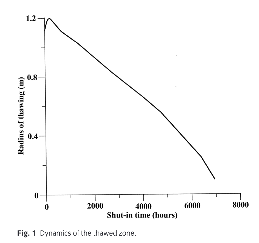
We obtained that h(t_c) = 1.12 m, Δt₀ = 113 hours and

Below we will neglect the difference between h_c and h_max. Refreezing of the thawed zone starts at the moment of time t = t₀ and ends at t = t_ep (Fig. 2).

We should note that only a part of the formation’s pore water changes to ice at 0°C. With further lowering of the temperature, phase transition of the water continues, but at steadily decreasing rates. The amount of unfrozen water is practically independent of the total moisture content for a given soil (Tsytovich 1975).

Time of the complete freezeback

It was assumed that the heat flow from the thawed zone to the thawed zone–frozen zone interface can be neglected. The results of hydrodynamical modelling have shown that this is a valid assumption (Kutasov 1999). In this case, the Stefan equation–energy conservation condition at phase change interface (r = h) is

Assuming the semi-steady temperature distribution in frozen zone (a conventional assumption), we obtain

where r_if is the radius of thermal influence during the freezeback period. The ratio D_f = r_if/h was determined from a numerical solution. A computer programme was used to obtain a numerical solution of a system of differential equations of heat conductivity for frozen and thawed zones and the Stefan equation (Kutasov 1999, 2006). It was found that

where I_f is the dimensionless latent heat density, L is the latent heat per unit of mass, c_f is the specific heat of the formation, ф is porosity, r_w is the water density, r_f is the formation density, r_w is the well radius, and l_f and a_f are the thermal conductivity and diffusivity of frozen formations, respectively.

From Eqns. 14–16 and the condition h(t₀) = h_max, we obtained (Kutasov 1999, 2006)

where H is the dimensionless radius of the thawing during shut-in.

From Eqn. 18 at h = r_w, we obtain the relationship for the duration of complete freezeback t_cf = t_ep – t₀ (Fig. 2).

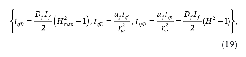
where t_epD is the dimensionless time of refreezing.

It is known that the electric resistivity of frozen sediments is affected by the freezing–thawing transition to a greater extent than the seismic velocities. Seismic velocities may increase by 2–10 times in transition to a frozen state, whereas the electrical resistivity may increase by 30 to 300 times in the same temperature interval (Hnatiuk & Randall 1977; Dobinski 2011). The dynamics of the thawed zone (the radius of thawing, Eqn. 18) while refreezing can, therefore, be monitored by geophysical methods (electric resistivity and seismic logs).

Method testing and discussion

Field example, Well Put River N-1, Alaska

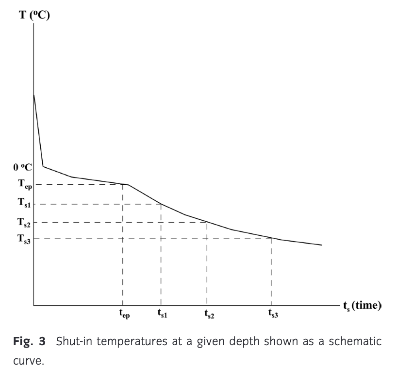
The input data and location of this well are presented in Table 2. This is a unique wellbore. Indeed, the first temperature log was taken after five days of shut-in and the last after three years of shut-in (Table 3). As we can see, the refreezing time increases with sufficiently high accuracy with the formation temperature increasing (Table 4). Figure 3 shows the results of calculations after Eqn. 1. It is clear that Eqn. 1 approximates the observed shut-in temperatures with sufficiently high accuracy.

The medium is a permafrost formation (sandstone). Only heat transfer by radial conduction is considered. The following parameters are introduced: the radius of the wellbore is 0.255, the thermal conductivity of frozen and unfrozen formations are l_f = 4.40 and l_un = 3.84 Wm⁻¹ K⁻¹, specific heat c_f= 950 and c_un =1138 Jkg⁻¹ K⁻¹, the density of sandstone is r_f = 2483 kg m⁻³, the density of water/ice is r_w = 1000 kg m⁻³, porosity is f = 0.09, and latent heat L = 334 960 J kg⁻¹ for water/ice. The latent heat density of the medium is c = Lr_wf = 334 960×1000×0.09 = 30×10⁶ Jm⁻³. The duration of the source disturbance is t_c. The phase change is assumed to be at 0°C. The temperature of drilling mud is assumed to be 8°C.

Estimation of the formation temperature

Recently, we suggested a new approach in predicting the undisturbed formations temperatures from shut-in temperature logs in deep wells (Kutasov & Eppelbaum 2018). The main features of the suggested method are the following: the refreezing of the thawed formations (around the wellbore) is completed; the temperature logs are taken after refreezing and the starting point in the well thermal recovery is moved from the end of well completion to the moment of time when the first shut-in temperature log was conducted. It is shown that after refreezing the further cooling of a well can be approximated by a constant (per unit of length) linear heat source. Hence, a modified Horner equation can be used for predicting the temperature of frozen formations for estimation of the formation temperature. A simple method to process field temperature data is presented. To demonstrate this approach, temperature shut-in time data for four depths from four wells in Alaska were successively used (Kutasov & Eppelbaum 2018).

We did not have an access to the drilling journal of this borehole to estimate the time of thermal disturbance, t_c (at a given depth), caused mainly by circulation of the drilling mud. For this reason, we consider thermal disturbance to start at the moment of time when the bit reached a given depth and the end of thermal disturbance is the moment when the drilling operations are completed. Then

where t_tot is the total drilling time, H_t is the vertical well depth and z is the current depth. Now we can consider that the period of time t*_c = t_c + t₀ as a new “thermal disturbance” period (t₀ = t_s1). Here t_s1 is the shut-in time for the first temperature log (Fig. 4). Therefore, for logs 2 and 3 the modified Horner equations are

From Eqns. 21 and 22, we can estimate the parameter B for a given depth and the formation temperature:

The results of calculations after Eqns. 22 and 23 are presented in Table 4.

The radius of thawing in the drilling period

Results of calculations after Eqns. 1, 2, 6–9 are presented in Table 5.

where t_D is the dimensionless drilling mud circulation time.

It is interesting to note that the dimensionless radius of thawing varies in narrow limits (Table 5). This can be explained by a combination of two factors: (1) the radius of thawing increases with depth (due to temperature increase with depth); (2) the time of mud circulation reduces with depth and the radius of thawing reduces with depth. The time of complete freezeback was calculated after Eqn. 19 (Table 6).

Conclusions

Drilling intermediate and deep wells in permafrost areas usually includes a warm mud application with unknown dynamics of the formation thawing around the wells. A new method based on the phase change (Stefan problem) around a cylindrical source is proposed. This method allows for the estimation of the radius of thawing during drilling and shut-in periods. Determining formation temperature and estimating the time of complete freezeback are illustrated with an example of field case.

Acknowledgements

The authors would like to thank two anonymous reviewers, who thoroughly reviewed the manuscript. Their critical comments and valuable suggestions were helpful in preparing this article.

References

1. Carslow H.S. & Jaeger J.C. 1959. Conduction of heat in solids. 2nd edn. Oxford: Oxford University Press.


2. Churchill S.W. & Gupta J.P. 1977. Approximations for conduction with freezing or melting. International Journal of Heat and Mass Transfer 20, 1251–1253, http://dx.doi.org/10.1016/0017-9310(77)90134-X.


3. Clow G.D. 2014. Temperature data acquired from the DOI/GTN-P Deep Borehole Array on the Arctic Slope of Alaska, 1973–2013. Earth System Science Data 6, 201–218, http://dx.doi.org/10.5194/essd-6-201-2014.


4. Dobinski W. 2011. Permafrost. Earth-Science Reviews 108, 158–169, http://dx.doi.org/10.1016/j.earscirev.2011.06.007.


5. Edwardson M.L., Girner H.M., Parkinson H.R., Williams C.D. & Matthews C.S. 1962. Calculation of formation temperature disturbances caused by mud circulation. Journal of Petroleum Technology 14(4), 416–426, http://dx.doi.org/10.2118/124-PA.


6. Eppelbaum L.V., Kutasov I.M. & Pilchin A.N. 2014. Applied geothermics. Heidelberg: Springer.


7. Harlan R.L. 1973. Analysis of coupled heat-fluid transport in partially frozen soil. Water Resources Research 9, 1314–1323, http://dx.doi.org/10.1029/WR009i005p01314.


8. Hasan A.R. & Kabir C.S. 1994. Aspects of wellbore heat transfer during two-phase flow. SPE Production & Facilities 9, 211–216, http://dx.doi.org/10.2118/22948-PA.


9. Hnatiuk J. & Randall A.G. 1977. Determination of permafrost thickness in wells in northern Canada. Canadian Journal of Earth Sciences 14, 375–383, http://dx.doi.org/10.1139/e77-038.


10. Jaeger J.C. 1961. The effect of the drilling fluid on temperature measured in boreholes. Journal of Geophysical Research 66, 563–569.


11. Judge A.S., Taylor A.E., Burgess M. & Allen V.S. 1981. Canadian geothermal data collection: northern wells 1978–80. Geothermal Series 12. Ottawa: Earth Physics Branch, Energy, Mines and Resources.


12. Kutasov I.M. 1987. Dimensionless temperature, cumulative heat flow and heat flow rate for a well with a constant bore-face temperature. Geothermics 16, 467–472, http://dx.doi.org/10.1016/0375-6505(87)90032-0.


13. Kutasov I.M. 1998. Melting around a cylindrical source with a constant wall temperature. In G.E. Tupholme & A.S. Wood (eds.): Mathematics of heat transfer. Pp. 213–218. Oxford: Clarendon Press.


14. Kutasov I.M. 1999. Applied geothermics for petroleum engineers. Amsterdam: Elsevier.


15. Kutasov I.M. 2006. Radius of thawing around an injection well and time of complete freezeback. Journal of Geophysics and Engineering 3, 154–159, http://dx.doi.org/10.1088/1742-2132/3/2/006.


16. Kutasov I.M., Balobayev V.T. & Demchenko R.Y. 1977. Metod “shivaniya” reshenii pri opredelenii ploskoi I zilindricheskoi granitzy razdela faz f zadache Stefana. (Method of “joining” of solutions in the determination of a plane and a cylindrical phase interface in the Stefan problem.) Engineering–Physical Journal (Inzhinerno-Geofizicheskii Zhurnal) 33, 148–152.


17. Kutasov I.M. & Eppelbaum L.V. 2003. Prediction of formation temperatures in permafrost regions from temperature logs in deep wells–field cases. Permafrost and Periglacial Processes 14, 247–258.


18. Kutasov I.M. & Eppelbaum L.V. 2017a. Time of refreezing of surrounding the wellbore thawed formations. International Journal of Thermal Science 122, 133–140, http://dx.doi.org/10.1016/j.ijthermalsci.2017.07.031.


19. Kutasov I.M. & Eppelbaum L.V. 2017b. Corrigendum to “Time of refreezing of surrounding the wellbore thawed formations.” International Journal of Thermal Science 124, 548.


20. Kutasov I.M. & Eppelbaum L.V. 2018. Utilization of the Horner plot for determining the temperature of frozen formations—a novel approach. Geothermics 71, 259–263, http://dx.doi.org/10.1016/j.geothermics.2017.10.005.


21. Kutasov I.M., Lubimova E.A. & Firsov F.V. 1966. Skorost’ vosstanovleniya temperaturnogo polya v skvazhinah Kol’skogo poluostrova. (Rate of recovery of the temperature field in wells in Kola Peninsula.) In: Problemy glubinnogo teplovogo potoka. (Problems of heat flux at depth.) Pp. 74–87. Moscow: Nauka.


22. Lachenbruch A.H. & Brewer M.C. 1959. Dissipation of the temperature effect of drilling a well in Arctic Alaska. U.S. Geological Survey Bulletin 1083-C, 74–109.


23. Lin S. 1971. One-dimensional freezing or melting processes in a body with variable cross-sectional area. International Journal of Heat and Mass Transfer 14, 153–156, http://dx.doi.org/10.1016/0017-9310(71)90146-3.


24. Lunardini V.J. 1988. Heat conduction with freezing or thawing. CRREL Monograph 88-1. Hanover, NH: US Army Corps of Engineers.


25. Melnikov P.I., Balobayev V.T., Kutasov I.M. & Devyatkin V.N. 1973. Geothermal studies in central Yakutia. International Geology Review 16, 565–568.


26. Ramey H.J.J. 1962. Wellbore heat transmission. Journal of Petrology Technology 14(4), 427–435.


27. Raymond L.R. 1969. Temperature distribution in a circulating drilling fluid. Journal of Petroleum Technology 21(3), 333–341, http://dx.doi.org/10.2118/2320-PA.


28. Romanovsky V.E., Gruber S., Instanes A., Jin H., Marchenko S.S., Smith S.L., Trombotto D. & Walter K.M. 2007. Frozen ground. In: UNEP global outlook for ice & snow. Pp. 181–200. Nairobi: Division of Early Warning and Assessment, United Nations Environment Programme.


29. Shiu K.C. & Beggs H.D. 1980. Predicting temperatures in flowing oil wells. Journal of Energy Resources Technology—Transactions of the ASME 102(1), 2–11, http://dx.doi.org/10.1115/1.3227845.


30. Sparrow S.W., Ramadhyani S. & Patankar S.V. 1978. Effect of subcooling on cylindrical melting. Journal of Heat Transfer 100, 395–402, http://dx.doi.org/10.1115/1.3450821.


31. Taylor A.E. 1978. Temperatures and heat flow in a system of cylindrical symmetry including a phase boundary. Geothermal Series 7. Ottawa: Earth Physics Branch, Energy, Mines and Resources.


32. Taylor A.E., Burgess M., Judge A.S. & Allen V.S. 1982. Canadian geothermal data collection: northern wells 1981. Geothermal Series 13. Ottawa: Earth Physics Branch, Energy, Mines and Resources.


33. Tien L.C. & Churchill S.W. 1965. Freezing front motion and heat transfer outside an infinite isothermal cylinder. A.I.Ch.E. Journal 11(5), 790–793, http://dx.doi.org/10.1002/aic.690110509.


34. Tsytovich N.A. 1975. The mechanics of frozen ground. Washington, DC: Scripta Book Co.


35. USGS 1998. Boreholes locations and permafrost depths. AK: U.S. Geological Survey. Accessed on the internet at https://nsidc.org/data/GGD223 on 5 April 2019.


36. Wang X., Wang Z., Deng X., Sun B., Zhao Y. & Fu W. 2017. Coupled thermal model of wellbore and permafrost in Arctic regions. Applied Thermal Engineering 123, 291–299, http://dx.doi.org/10.1016/j.applthermaleng.2017.05.186.


37. Wu Y.S. & Pruess K. 1990. An analytical solution for wellbore heat transmission in layered formations. SPE Reservoir Engineering 5, 531–538, http://dx.doi.org/10.2118/17497-PA.