This article is published under a Creative Commons license and not by the author of the article. So if you find any inaccuracies, you can correct them by updating the article.

Application of remotely piloted aircraft systems in observing the atmospheric boundary layer over Antarctic sea ice in winter


Marius O. Jonassen
Andreas Scholtz
Timo Vihma
Astrid Lampert
Gert König-Langlo
Christof Lüpkes
Priit Tisler
Barbara Altstädter
Published: Oct. 8, 2015
Latest article update: Aug. 19, 2023
This article is published under the license


Abstract
The main aim of this paper is to explore the potential of combining measurements from fixed- and rotary-wing remotely piloted aircraft systems (RPAS) to complement data sets from radio soundings as well as ship and sea-ice-based instrumentation for atmospheric boundary layer (ABL) profiling. This study represents a proof-of-concept of RPAS observations in the Antarctic sea-ice zone. We present first results from the RV Polarstern Antarctic winter expedition in the Weddell Sea in June–August 2013, during which three RPAS were operated to measure temperature, humidity and wind; a fixed-wing small unmanned meteorological observer (SUMO), a fixed-wing meteorological mini-aerial vehicle, and an advanced mission and operation research quadcopter. A total of 86 RPAS flights showed a strongly varying ABL structure ranging from slightly unstable temperature stratification near the surface to conditions with strong surface-based temperature inversions. The RPAS observations supplement the regular upper air soundings and standard meteorological measurements made during the campaign. The SUMO and quadcopter temperature profiles agree very well and, excluding cases with strong temperature inversions, 70% of the variance in the difference between the SUMO and quadcopter temperature profiles can be explained by natural, temporal, temperature fluctuations. Strong temperature inversions cause the largest differences, which are induced by SUMO’s high climb rates and slow sensor response. Under such conditions, the quadcopter, with its slower climb rate and faster sensor, is very useful in obtaining accurate temperature profiles in the lowest 100 m above the sea ice.
Keywords
Antarctic, polar meteorology, boundary layer meteorology, Remotely piloted aircraft systems, unmanned aerial vehicles, Weddell Sea
The vertical structure of, and processes in, the atmospheric boundary layer (ABL) play an essential role in the Antarctic climate system. To better understand the system, in situ observations are very valuable, enabling validation and further improvement of parameterizations for numerical weather prediction and climate models.
Very few meteorological observations have been available from Antarctic sea ice in winter. The first set of meteorological observations throughout an Antarctic winter was made when de Gerlache’s ship the Belgica was trapped in sea ice at 72°S, 90°W during the winter of 1898 (King & Turner 1997). The period of the “heroic age” of Antarctic exploration included two (unplanned) overwintering expeditions in the interior of the Weddell Sea: Filchner with the Deutschland in 1912 and Shackleton with the Endurance in 1915. The first intentional scientific drifting ice station in the Weddell Sea was established in 1992 by a joint effort of the United States and Russia (Gordon et al. 1993). This yielded meteorological data based on tower measurements and radiosonde soundings during four months in the austral fall and winter (Andreas 1995; Andreas & Claffey 1995; Andreas et al. 2000; Andreas et al. 2004, 2005). This is the most extensive meteorological data set so far collected from the Antarctic sea-ice zone and is still used to validate models and reanalyses (Tastula et al. 2012; Tastula et al. 2013).
The RV Polarstern first spent the winter in the pack-ice zone of the Antarctic in 1986, serving as a platform for the first detailed survey of the structure and dynamics of water, ice and the lower atmosphere in the Weddell Sea south to 76°S (Hempel 1988). Another cruise of the research vessel followed in 1989 with the Winter Weddell Gyre Study (König-Langlo et al. 1991; Haas et al. 1992; Wamser & Martinson 1993; König-Langlo et al. 2010a, b). Meteorological processes and air–ice–ocean interaction in the Antarctic sea-ice zone in winter have also been studied on the basis of drifting buoys (Vihma & Launiainen 1993; Launiainen & Vihma 1994; Kottmeier & Sellman 1996; Vihma et al. 1996), supported by model experiments (Valkonen et al. 2008). Buoy observations are, however, limited to the lowest metres of the atmosphere.
During recent years, the rapid development of remotely piloted aircraft systems (RPAS), also called unmanned aerial vehicles, has significantly extended the measurement capabilities in ABL research (e.g., Reuder et al. 2012). Traditional measurement methods of the ABL, such as masts, lidars and sodars, are typically rather expensive and infrastructurally demanding, particularly in remote areas and in harsh, polar conditions. Developments in microelectronics and miniaturization of sensors and components allow an ever-increasing utilization of very small, lightweight and flexible RPAS for scientific purposes. The first use of RPAS in the Antarctic took place in December 2007, when scientists from the British Antarctic Survey operated the meteorological mini-aerial vehicle (MMAV) over the Brunt Ice Shelf and adjacent Weddell Sea. The first RPAS measurements over the Antarctic sea-ice zone were carried out in September 2009 (Cassano et al. 2010; Knuth et al. 2013; Knuth & Cassano 2014), followed by two campaigns in 2012 (Cassano 2013).
In this paper, we explore the feasibility of combining temperature observations from radiosonde soundings and a set of surface- and ship-based platforms with RPAS measurements for frequent profiling of the polar ABL. We do so by analysing measurements carried out during the RV Polarstern cruise in winter 2013 in the ice-covered Weddell Sea, Antarctic. During the cruise, two surface- and ship-based automatic weather stations (AWS) were operated along with three different RPAS platforms. Two of the RPAS, known as the small unmanned meteorological observer (SUMO) and MMAV, both fixed-wing, have been utilized several times before in polar environments. The third, an advanced mission and operation research (AMOR) quadcopter, has never before been used under such conditions.
In this paper, we first evaluate the RPAS data against the above-mentioned measurements. Second, we compare the SUMO to the new AMOR quadcopter for measuring temperature profiles up to 100 m above the sea ice. Our motivation for using the quadcopter is a more accurate sampling of fine-scale ABL structures, such as sharp temperature gradients, especially close to the surface in terms of surface-based inversions, since these are notoriously difficult to capture using fast ascending RPAS platforms like the SUMO, as will be demonstrated herein.
This study should be regarded as proof-of-concept and the emphasis will be on evaluating the RPAS performance and describing challenges with operations in harsh, polar conditions. The main focus of this paper will be on vertical profiles of temperature in the ABL and technical aspects of these measurements. Other meteorological parameters, such as the wind vector and air humidity and related processes, will be addressed in forthcoming papers.
Observations
Study area and ice stations
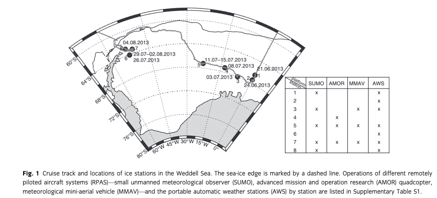
The RV Polarstern winter expedition ANT-XXIX/6 started from Cape Town, South Africa, on 8 June 2013. In the beginning, the cruise track (Fig. 1) followed the Greenwich Meridian southwards. Close to the Antarctic continent, the ship headed north–west and crossed the Weddell Sea, reaching Punta Arenas, Chile, on 12 August 2013. The first ice station was established on 21 June and the last on 4 August. Altogether, eight ice stations were set up (Fig. 1).
Remotely piloted aircraft systems
The vertical profiles of the ABL during this expedition were obtained by using three different types of RPAS. Firstly, the fixed-wing platform SUMO, designed as a “recoverable radiosonde” for ABL research, was employed. SUMO is based on a commercially available construction kit called FunJet, from Multiplex (Bretten-Gölshausen, Germany). It has a wingspan of 0.8 m and when fully equipped has a take-off weight of around 800 g with a payload capacity of 200 g. Each flight lasts up to 30 min and the maximum reachable altitude is around 4 km. The cruising speed is around 18 m s−1, and the maximum wind speed for operations is around 15 m s−1. The aircraft is equipped with meteorological sensors for the measurement of temperature (PT-1000 M 222, Heraeus, Hanau, Germany), humidity (SHT 75, Sensirion, Staefa, Switzerland) and atmospheric pressure (MS5611, Measurement Specialities, Hampton, VA). Wind speed and wind direction are estimated using an algorithm that takes into account the ground speed and flight azimuth data from the on-board global positioning system (GPS) (Mayer et al. 2012). Autonomous operation of the aircraft is possible via an autopilot system from Paparazzi (ENAC 2008), allowing the operator (a) to predefine complex flight missions and (b) to modify the flight plan at any time in-flight using the 2.4-GHz bidirectional data link. The typical flight pattern of SUMO for boundary layer profiling is a helical track, consisting of manual take-off and manual landing (Jonassen 2008). Fully autonomic profiling is preceded by an aircraft functionality check at a safety altitude, at approximately 100 m. During the functionality check, the aircraft is kept in a circular flight path at a constant altitude, while important parameters such as attitude control, GPS signal, telemetry signal and battery are checked using the ground control station. After this check, the aircraft is sent down to the lowest safe altitude (typically 30 m) followed by a climb to the desired maximum altitude whilst keeping the aforementioned helical flight pattern. Depending on the synoptic situation, two main measurement strategies were used: (a) two up-and-down profiles with a maximum altitude of 1100 m during one flight and (b) one up-and-down profile with a maximum altitude of 1700 m during one flight. The meteorological parameters from SUMO, except wind, were interpolated to 1 Hz. More information about the airframe and technical specifications of the meteorological sensors has been presented by Reuder et al. (2008, 2009).
The MMAV was developed at the Institute of Aerospace Systems, Technical University Braunschweig. It is based on the unmanned Carolo T200 aircraft, with a wingspan of 2 m and a maximum take-off weight of 6 kg, including 1.5-kg payload (Spieß et al. 2007). The MMAV endurance is up to 60 min with a cruising speed of 22 m s−1. During the cruise, the MMAV was launched by a winch system fixed in the snow and ice surface. It operates under the control of the Mavionics (Braunschweig, Germany) MINC autopilot system (e.g., Martin et al. 2011). It is programmed prior to the flight, and the waypoints in three dimensions can be updated during the mission by a telemetry link from the ground-based station. The meteorological sensor package of the MMAV was developed at the Institute of Aerospace Systems. An HMP 50 resistance thermometer (Vaisala, Vantaa, Finland) with high accuracy but slow response time (in flight about one second) is used. The same HMP 50 provides air humidity data rather slowly but with good accuracy over the temperature range of interest. The wind vector in the airframe coordinate system is measured by a miniaturized, five-hole probe, developed and manufactured by the Institute of Fluid Dynamics, Technical University Braunschweig. In vertical profiles (at a typical climb rate of 3 m s−1), a vertical resolution of 10 cm can be achieved (Martin et al. 2011). During the RV Polarstern campaign, the MMAV was used for profiling the ABL up to 1400 m and for deriving turbulent properties on straight and level legs (turbulence analyses are not included in this article). All meteorological parameters from the MMAV were sampled at 100 Hz. Functionality checks of the system were performed before take-off.
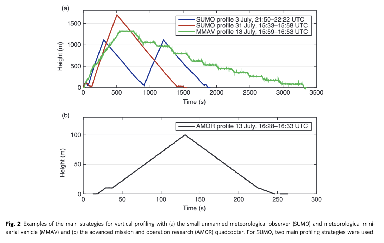
Figure 2 shows an example of typical flight patterns for ABL profiling. The MMAV profile consisted of a manually flown, fast ascent up to around 500 m followed by a climb controlled by the autopilot to the maximum altitude of the mission. Afterwards, a horizontal leg in the form of a rounded square was performed to calibrate the wind components before the slow descent began including several wind calibration legs at different altitudes. Note the safety altitude at 100 m in the flight pattern for SUMO and the corresponding one at 20 m for the quadcopter. These flight patterns were designed to obtain as much information as possible on the structure of the ABL, not particularly for comparisons of SUMO, MMAV and the quadcopter.
An AMOR quadcopter was used in order to get more information from the lowest 100-m layer of the atmosphere. It is developed at the University of Applied Sciences Ostwestfalen-Lippe and utilizes a multi-level structure, enabling enhanced accuracy of the position and the sensor data (Dünnermann & Wrenger 2011). The quadcopter is based on a composite airframe and is equipped with four propellers with electric motors, providing a payload capacity of up to 2 kg. The endurance of the quadcopter is up to approximately 30 min, depending on the battery package and the payload. The vertical climb rate is adjustable and was set to 0.8 m s−1 during the RV Polarstern cruise. The quadcopter’s meteorological sensor package is mounted on top of a vertical boom pointing above the platform to reduce influence from the rotor blades (see Supplementary Fig. S1). The package comprises a pressure sensor, standard sensors for temperature and humidity: an HYT 271 combined humidity and temperature module (Innovative Sensor Technology, Las Vegas, NV), PT-1000 temperature sensor (Heraeus) and P-14 Rapid Capacitive Humidity Sensor (Innovative Sensor Technology), a fast thermocouple temperature sensor and an infrared surface temperature sensor. All meteorological parameters from the quadcopter were sampled at 10 Hz. The data acquisition system enables on-board data storage as well as continuous data monitoring on the ground control station during the flight. Carrying out flight missions with the quadcopter is possible in manual (stabilized), loiter and autonomous mode. During this campaign, the fully autonomous mode was used in all our flight missions, including a predefined flight scenario with automatic take-off and landing procedures. Supplementary Fig. S1 shows all three RPAS during operation.
Additional meteorological measurements
Routine meteorological observations are performed by the Meteorological Observatory of RV Polarstern during all cruises (König-Langlo et al. 2006) and these data are also available for the present cruise (König-Langlo 2013a). Standard synoptic observations were carried out every three hours (König-Langlo 2013b). In addition, air temperature measurements were made at 29-m height and wind measurements at 39-m height, both with a one-minute interval. Upper air soundings with Vaisala radiosondes were carried out on a daily basis at around 11 UTC, providing profile measurements of pressure, temperature, relative humidity and the wind vector (König-Langlo 2013c). All these data are available at www.pangaea.de/search?q=Campaign:ANT-XXIX/6. Data from the airborne instruments and routine measurements were supplemented by meteorological observations from a small portable weather mast, deployed on the ice during the ice stations. Air temperature was measured at the heights of 0.1, 0.5 and 2 m. Wind speed and direction were measured at the height of 2 m. The measurements were obtained using Aanderaa (Bergen, Norway) and MSR145 (MSR Electronics, Seuzach, Switzerland) sensors/data logging systems. Details about the airborne flight missions and weather mast measurements are given in Supplementary Table S1.
Results
The operation of the RPAS was restricted to ice stations because take-off and landing were not permitted from the deck of the vessel. However, finding a suitable landing strip on rough, ridged sea ice often proved difficult, especially for the MMAV, which used a winch system for take-offs and landed directly on the fuselage. Although the weather conditions were not always favourable for flying, SUMO was operated on nine different days (hereafter referred to as episodes) during a total of five ice stations; more than 50 successful flights were performed. The MMAV was operated during eight days with a total of 11 flights.
For a first evaluation of the SUMO and MMAV vertical profiles, we compare them with RV Polarstern radiosonde data. Figure 3a presents average vertical temperature profiles from the SUMO and radiosondes. Overall, the mean difference between average profiles of the two platforms is within 0.76 K. The average radiosonde profile is less smooth than the average SUMO profile, which is to be expected since we have considered here radiosonde profiles measured only during the ice stations, and they were far fewer (10) than the SUMO profiles (69). Some discrepancy can also be explained by an irregular schedule of observations, resulting in up to several hours between SUMO flights and radiosonde measurements.
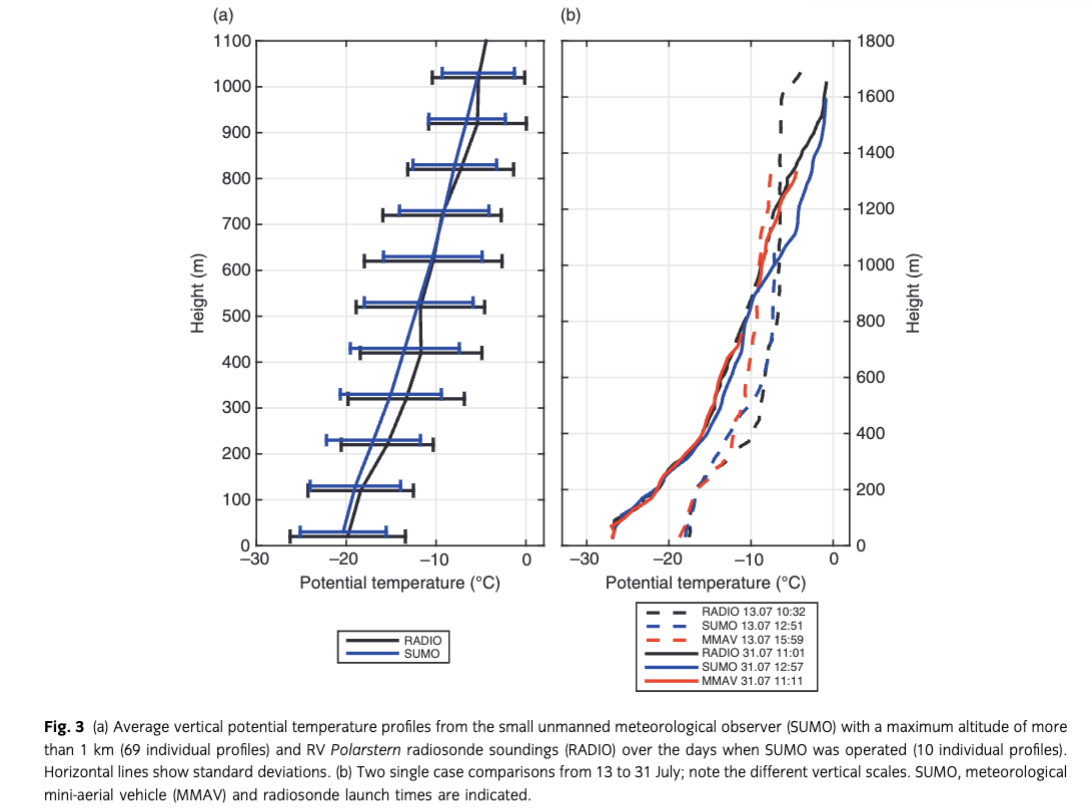
Two single cases with small timing difference (less than two hours) are compared in Fig. 3b. In both cases, the SUMO profiles were made up to an altitude of 1700 m and both situations included a strong inversion in the lowest part of the boundary layer. The temperature profiles obtained by SUMO agree with the radiosonde observations reasonably well, within an average difference of −0.7 K (13 July) and 1.0 K (31 July). An MMAV average profile is not presented here because there were only a very few vertical profiles to sufficient altitude. However, two single and most representative MMAV profiles are shown in Fig. 3b. The MMAV profiles coincide with RV Polarstern soundings rather well, with an average difference of −1.7 K (13 July) and 0.1 K (31 July). The differences between RPAS and radiosonde measurements are most likely explained by the time difference between the profiles and/or smaller calibration offsets. Such offsets will be investigated in further detail in the Discussion section.
The comparison of RPAS profiles with RV Polarstern radiosonde soundings showed that the overall agreement was quite good, but the distance in time and space between the profiles did not allow a detailed comparison and identification of measurement problems. The SUMO and quadcopter, however, were operated within small distances in time and space, which allows for a more comprehensive comparison of the two.
The AMOR quadcopter was used during three ice stations (five episodes), resulting in 24 profile flights up to 100-m height. It became evident that interpretation of the temperature and humidity profiles from the AMOR standard sensors requires special correction due to uncertainties related to the slow response time of those sensors. As will be demonstrated below, the fast thermocouple temperature sensor, however, shows a very good agreement with independent temperature measurements at the height of 2 m (in the weather mast) and 29 m. Therefore, only measurements from the fast thermocouple temperature sensor will be considered in this study.
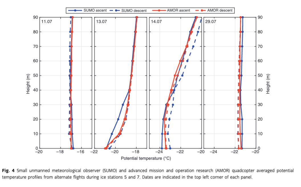
During ice stations 5 and 7 (see Supplementary Table S1), SUMO and the quadcopter were operated sequentially, which allows a comparison of the two. We have here matched their profiles in time, where a match is defined as a maximum of 20 min difference between the end of one profile and the start of the next. In the matching process, we treat each ascent and descent profile individually, implying that each RPAS flight yields two profiles. This gives us a total of 63 matches for the four days they were operated sequentially. In the following, we will only consider temperature, as the quadcopter did not measure wind and the humidity measurements proved rather unreliable from both platforms.
Profiles from SUMO and the quadcopter averaged first at height intervals of 10 m and thereafter over each of the four days with sequential operations are presented in Fig. 4. Evidently, there is a rather strong day-to-day variability in the vertical thermal structure of the lowest 100-m atmosphere, and this is reflected in how the RPAS profiles match. Starting with 11 July, we observe a slight decrease in potential temperature with height up to around 20 m, followed by a close to constant potential temperature aloft. We therefore have statically unstable conditions close to the surface with a statically neutral layer farther aloft. The different RPAS potential temperature profiles are almost not discernable on this day. On 13 July, the whole probed atmospheric layer is statically stable, with the strongest stratification found below 40 m, indicating the presence of a surface-bound inversion for both the true and potential temperature. Within this inversion layer, there is a relatively large difference between the SUMO ascent and descent profiles (up to 1 K), and the sharpening of the potential temperature gradient towards the ground seen in the descent profile is not present in the ascent profile. The AMOR ascent and descent profile pairs from 13 July, however, match each other very well. On 14 July, the boundary layer within the lowest 100 m is characterized by a very weak potential temperature gradient below 30-m height, with an increasing potential temperature above. Like the situation on 13 July, there is a relatively large difference between the SUMO ascent and descent profiles, but on this day the difference extends through the whole vertical column investigated. Again, the AMOR ascent and descent profiles match very well. The days 29 July and 11 July resemble one another in having largely neutrally stratified potential temperature profiles. The difference between the SUMO ascent and descent profiles, however, is somewhat larger, but still within a mere 0.5 K.
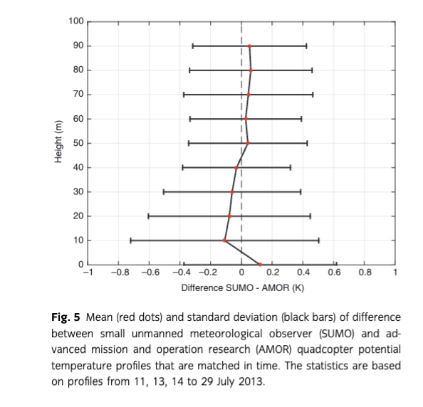
Summary statistics of the difference between SUMO and AMOR profiles matched in time for all four days is shown in Fig. 5. In general, the two RPAS match very well with standard deviations of the difference under 0.7 K and a vertically averaged difference very close to 0 K (SUMO being slightly warmer).
From the above analysis, it appears that the difference between the RPAS profiles depends on the vertical temperature structure of the investigated atmospheric column. In the following, we will consider in more detail two cases with distinctly different conditions, one with a weak near-surface temperature gradient (11 July, 22:36–23:22 UTC) and one with a strong near-surface temperature gradient (13 July, 18:59–19:35 UTC).
The day 11 July started with weak to moderate westerly winds, gradually turning northerly with decreasing wind speed (Fig. 6). The lower troposphere had a fairly weak potential temperature gradient this day. Figure 7 shows a set of matched AMOR and SUMO temperature profiles within the considered time frame. The SUMO profiles contain a higher number of samples below 100 m, which is caused by the initial SUMO flight check at 100 m above ground (see Fig. 2a). The result can be seen in the SUMO raw ascent profile, which obviously is sampled several times and also contains some irregularities. Some of these irregularities can also be explained by a less-than-optimal attitude control during manual flight mode.
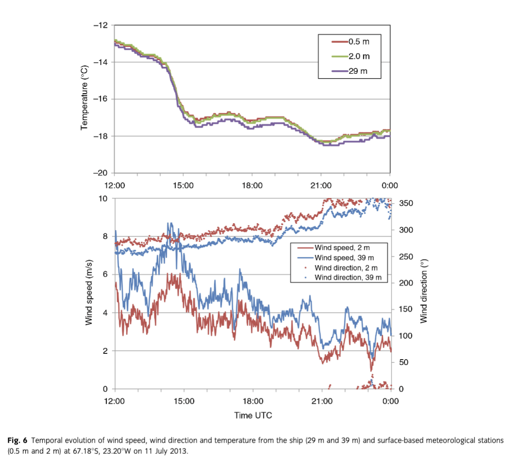
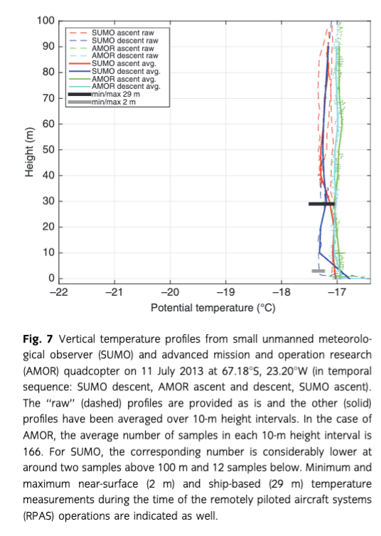
Nevertheless, the profiles from the two platforms match each other very well and there is only a slight difference in temperature amounting to around 0.3 K at the most. Except the SUMO ascent profile, the presented “raw” ascent and descent profiles are hardly discernable from the 10 m height-averaged profiles, indicating a low variability within the 10-m intervals in this case and the two RPAS also match fairly well the minimum and maximum shipborne (29 m) and surface-based (2 m) temperature measurements.
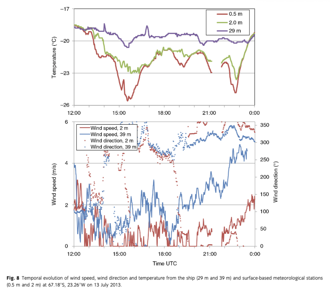
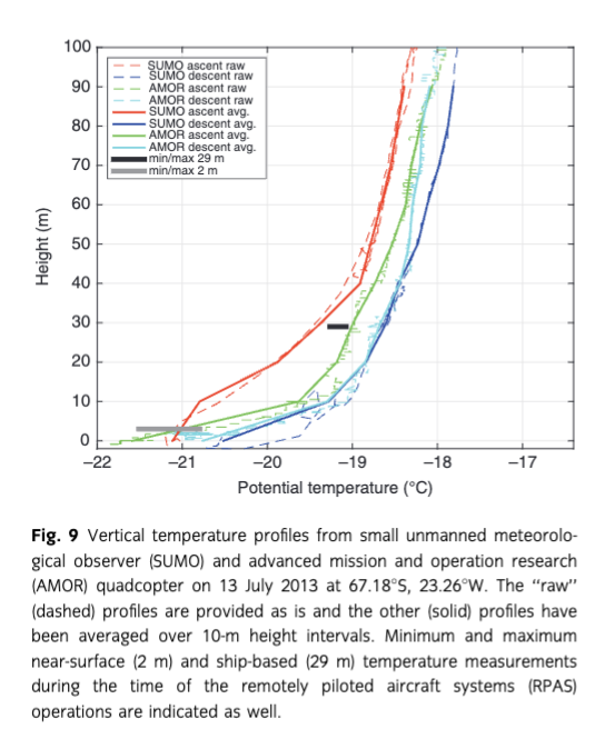
On 13 July, there were generally weak winds (less than 5 m s−1) with no well-defined wind direction over our measurement area (Fig. 8). The potential temperature gradient in the lower ABL was relatively steep throughout most of the day with a rather large variability in temperature close to the surface as seen in the AWS data. In this case (Fig. 9), there are larger discrepancies between the profiles from the two RPAS than in the previous case of 11 July. The SUMO ascent profile is through most of the probed atmospheric layer 0.5 to 1 K colder than the other profiles. This cold bias is also symptomatic for the other SUMO ascent profiles in the strongly stable surface conditions of 13 July (Fig. 4), and in the presented case the bias magnitude is around the average (bias varying from case to case). A corresponding, but smaller warm bias is found in the SUMO descent profile. These systematic warm and cold biases are caused by the high ascent and descent rates of the SUMO aircraft (typically 2–5 m s−1), combined with a relatively slow sensor response. Like in the “raw” SUMO profiles from 11 July, on this day we can see some irregularities.
To compare the RPAS profiles against the ship-based measurements, all RPAS GPS height data points within 29±5 m a.s.l. were identified and an average temperature was calculated for these data points. This was done separately for the RPAS ascent and descent profile parts. The comparison was made for simultaneous (±2 min) ship and RPAS data. The near-surface estimates for the RPAS were calculated over a height interval of 0 m a.s.l. ±5 m. Negative altitudes were included to account for smaller GPS height inaccuracies that were observed to occur occasionally in both RPAS. These RPAS measurements were then in turn compared to the averaged surface-based measurements (2 m) in the same way as for the ship-based instruments. The results are shown in Fig. 10.
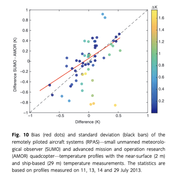
On the average, the RPAS temperature measurements are a bit colder than the surface- and ship-based measurements and the standard deviations are small at 0.3 K or lower (Fig. 10). Except for the SUMO ascent 29 m statistics, the best matches are found between the quadcopter and the reference measurements. During operation, the horizontal separation between the RPAS and the ship was of the order of 100 m.
Discussion
The RPAS add a detailed picture of the vertical temperature profile of the ABL to the rare radiosonde data. The data reveal highly resolved structures, which cannot be captured with the rather coarse resolution of the soundings. A further advantage of RPAS is the flexibility to probe the ABL consecutively at short intervals, which allows retrieving the temporal development on the local scale.
In summary, we find that the added value of the AMOR quadcopter in profiling the lower ABL depends on the vertical temperature gradient. Under neutral or close-to-neutral, near-surface temperature stratifications, SUMO and the quadcopter perform about equally well by judging how well their pairs of ascent and descent profiles match. Under strong temperature stratifications, however, the quadcopter reproduces more realistic near-surface temperature profiles, with a generally closer match between ascent and descent profiles and with fewer profile irregularities (as described in the Results section) than SUMO.
There are various methods for overcoming problems with the slow sensor response seen in the SUMO data. Some of the simplest methods involve shifting ascent profiles downwards and descent profiles upwards in the profile post-processing by imposing a time offset (e.g., Cassano 2013). The vertical shift may be estimated by identifying the shift that gives the lowest average difference between pairs of ascent and descent temperature profiles. Doing so for the SUMO profiles at hand, it appeared that the ascent and descent profiles are, on average, shifted vertically by 10 m with respect to each other (not shown). This number varies from flight to flight; for example, in the flight data presented in Fig. 9, it is at least twice that, suggesting the presence of additional sources for profile disparities. Using the following equation (Jonassen 2008), one can make a rough estimate of the sensor response time where ΔHasc–des is the height shift, τs is the time constant for the temperature sensor and Vasc and Vdes are vertical ascent and descent rates, respectively. Inserting a typical height shift of 10 m and a vertical (ascent and descent) speed of 2.5 m s−1, Eqn. 1 yields a τs of two seconds for the SUMO temperature sensor. It is evident that a lower ascent and/or descent rate will reduce the time lag/height shift, and operating SUMO with, for example, a 1 m s−1 vertical speed (close to that of the quadcopter) in both directions would, by Eqn. 1, give a theoretical shift of only 4 m. Such a slow vertical speed is, however, not feasible when high-altitude profiles are desired, since it will significantly reduce the maximum reachable altitude due to limited battery capacity.
There are also more sophisticated numerical algorithms for time lag correction that take the sensor response time into account (e.g., Miloshevich et al. 2004). This type of a method has previously been applied to SUMO profiles with some degree of success (Jonassen 2008). In the present study, we have chosen not to correct the SUMO profiles for time lag since the profile parts of most interest here are found below 100 m and this is where the strongest profile irregularities are found. Such irregularities are especially problematic to correct as outlined by Jonassen (2008). For future studies, a more sophisticated correction algorithm should be used, or better, a new and faster sensor should be implemented, eliminating the need for any time lag correction. Also, it is clear that faster humidity sensors are needed for all three RPAS, as the current ones have time constants of at least 10 s (a rough estimate using Eqn. 1). Furthermore, humidity sensors get slower with lower temperatures as discussed by Jonassen (2008), among others, so a correction is not straightforward over a large span of temperatures.
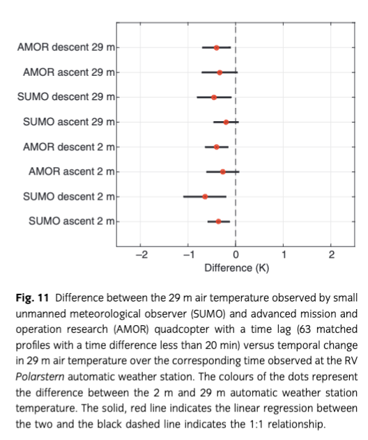
In addition to the above discussed sensor- and platform-related factors inducing differences between the RPAS profiles, natural temperature variability in time and space may also be expected to cause profile disparities. SUMO and the quadcopter were operated by the same team (two people), and they could not operate the two platforms simultaneously. The solution was sequential flights and some time separation, although small, did occur. The operation location, however, was practically unchanged, except by a few tens of metres because of ice floe drift and a slight offset in the horizontal since SUMO was operated with a helical flight pattern and the quadcopter ascended and descended over the same spot. We therefore expect the impact of spatial variability on the profile disparity to be low. Temporal variability can, however, be expected to be a more significant cause of profile disparity. Some light can be shed on the importance of this latter factor by comparing the difference between the time-matched RPAS profiles and the variability in the AWS temperature between the flights. Figure 11 shows a scatter diagram of the difference between the 29 m temperatures observed by SUMO and AMOR and the temporal difference in the 29 m AWS temperature between the SUMO and AMOR observation times. From this diagram, we can see that (a) the natural, temporal temperature variability and the difference between the matched RPAS profiles are generally of the same order and (b) there is a positive correlation between the two. Excluding the outliers, we get a correlation coefficient (r) of 0.84, which gives an r2 of 0.7. This means that 70% of the variance in the difference between the 29-m RPAS temperatures can be explained by natural, temporal temperature variability at 29 m. A further investigation of the above-mentioned outliers reveals that these are associated with large differences between the 29 m and 2 m AWS temperatures (colour codes in Fig. 11, indicating strong temperature stratification. These outliers are all from 13 July. In fact, all points with a vertical temperature gradient larger than 0.8 K are from that date. When including all data points, r2 becomes 0.24.
Another area where the RPAS could be improved is the implementation of an icing detection system. Light-to-moderate icing occurred on the fuselages, sensors, wings, control surfaces and propellers on the MMAV and SUMO on a few occasions (four flights for MMAV and five for SUMO). The icing did not result in any crashes, but it did degrade the flight performance, which in the case of SUMO was most notable in the achieved climb rate. For the MMAV, having a longer endurance than SUMO thus giving ice more time to build up, the symptoms were in several cases stronger. The icing was especially strong at one occasion, when a racetrack pattern was flown at night. At that occasion, the aircraft flight performance when operated in autonomous mode was not noticeably degraded. During the manual landing procedure, however, the controllability was extremely reduced and only a skilled pilot prevented the aircraft from taking damage under the landing. In the post-flight inspection of the MMAV aircraft, its weight had increased by 690 g, which is equivalent to about 11.5% of its original take-off weight. In this case, most of the ice had accumulated on the leading edges of the wings, on the propellers and especially the elevator. In addition, milder cases of icing occurred with the MMAV reducing the telemetry signal quality. During the icing events, the measured relative humidity from SUMO was between 80 and 90%, indicating an atmosphere close to saturation.
Furthermore, near-surface temperatures frequently below −20°C generated a need to heat the aircraft batteries and RPAS remote controls before operation. In the case of SUMO and the quadcopter, this was solved using a combination of heating pads and a small, heated storage box powered by a 12 V car battery that were brought on to the ice during operations. Other than that, the SUMO and quadcopter fuselages with otherwise complete sets of on-board electronics worked flawlessly even after lying hours on the sea ice in temperatures down to −30°C. The MMAV has larger batteries (less self-heating during flight) and its endurance is longer than the other RPAS, so pre-heating and preventing of cooling of the batteries is of even larger importance than for the other systems. This was solved by keeping the fuselage including pre-heated batteries and avionics with meteorological sensors in an insulating transport box up until each flight. On some occasions, an additional temperature-related problem occurred with the motors’ electronic speed controllers. If they were exposed to the environment with temperatures below −15°C for more than 15 min, the automatic pre-flight throttle control position calibration did not work properly. In these events, the engine nacelles were heated with hand warmers for two minutes and the activation procedure for the propulsion system was repeated afterwards without any problems and influences on the flight performance, even under temperatures below −30°C. The reason for this behaviour might be a temperature-sensitive oscillator for pulse width modulation signal measurement on the electronic speed controllers, which has not been seen with previous versions of the system. Other than the above-mentioned deficiencies and an increased need for maintenance due to ageing electronics, the technical reliability of the Carolo T200 airframe was on a high level. Given that the outlined procedures were followed, the system performed at a level similar to that seen previously during campaigns at the mid-latitudes (Martin et al. 2011).
This work makes it clear that the quadcopter represents a valuable addition for probing the lower polar ABL. A faster sensor in the SUMO system would presumably alleviate problems with time lag, but the sub-optimal flight pattern during landing and take-offs is hard to avoid and would probably still cause challenges in obtaining coherent profiles of the lowermost parts of the ABL. Then the quadcopter is highly useful in that it operates with a very low and consistent ascent/descent rate all the way from the ground and up. Another advantage with the quadcopter is its ability to take-off from virtually any surface large enough to fit it (ca. 80×80 cm). It can take-off and land on ridged sea ice and other difficult surface types with relative ease. In fact, rough landing conditions were the reason why only the quadcopter was operated on 8 July.
The synoptic situation and the vertical structure of the ABL were rather varying during the ice stations. The number of available profiles does not allow a detailed climatological analysis of the ABL structure. In two out of the nine episodes (21 June and 14 July) distinct and strong, surface-based temperature inversions were observed with depths reaching 400 m. Their strength was more than 10 K, which is similar to values obtained in the Central Arctic winter by drift stations (Kahl et al. 1999). A majority of the episodes, however, had a more complex boundary layer structure with multiple, but essentially weaker, inversion layers similar to observed profiles over the ice-covered western Weddell Sea (Andreas et al. 2000) and in the area of Spitsbergen, in the Arctic (Reuder et al. 2008; Vihma et al. 2011). Stable stratification is often associated with low-level jets, usually embedded in the inversion layer, as Andreas et al. (2000), Jakobson et al. (2013) and others have detected over sea ice. Evident occurrence of low-level jets during SUMO missions was observed infrequently, due to technical limitations, restraining flights in case of strong winds.
Concluding remarks
We have presented observations of air temperature profiles over Antarctic sea ice in winter. Observations were made in the interior of the Weddell Sea during an expedition with RV Polarstern in June–August 2013. A novel aspect of this campaign was the combined use of RPAS, radiosonde soundings, ship observations and a small portable weather mast. Three different RPAS systems were used sequentially, complementing each other. The fixed-wing SUMO and MMAV were operated for measurements up to altitudes of 1.7 km, while the AMOR quadcopter was operated in order to get more detailed measurements from the lowest 100-m layer. Having a faster temperature sensor and a slower and more consistent ascent/descent rate, the quadcopter clearly adds value in producing more accurate temperature profiles compared to the SUMO system under conditions with very strong vertical temperature gradients. In addition, the quadcopter performs single-column profiles with fully automatic landings and take-offs. Mainly on account of its size, the MMAV proved to be somewhat more challenging for operations from the predominantly rough sea ice than the other RPAS. Nevertheless, like the SUMO, the MMAV produced high-quality temperature profiles that compared favourably against the available radiosonde data. In addition, the MMAV provided measurements of turbulent fluxes. Presenting these data is, however, not within the scope of this article.
All three RPAS demonstrate several advantages in performing highly resolved temperature profiles compared to recognized radiosonde and tethersonde systems. In comparison with surface-based remote sensing methods like sodars and lidars, RPAS are more flexible and can be operated according to changing conditions, for example, above leads in the sea-ice zone, or upwind and downwind from the ship. Modern RPAS are becoming easy to operate. Only rather short training (as in the case of SUMO and AMOR) is required, enabling system operation exclusively by scientists without a need for experienced specialists in RPAS technology. Requirements for suitable landing and take-off areas are very modest, particularly for the AMOR quadcopter. This makes the utilization of these RPAS very attractive, especially in remote polar environments with very limited infrastructure. The RPAS discussed here can be characterized by a notable cost-efficient performance. Although larger RPAS have greater endurance and payload capacity, they also need more skilled labour and the price of larger systems is an order of a magnitude higher.
The weather conditions during the expedition and ice stations were not always favourable for flying. The most significant factor limiting operation was strong wind (over 10 m s−1) for SUMO and the quadcopter and unfavourable, rough ice conditions for landing the MMAV. Despite the RPAS being equipped with an inertial measurement unit for airframe attitude control, poor visibility due to low foggy clouds was another rather serious restraint for flying. Ice formation on the RPAS wings and propeller blades was the third problem causing shorter flying time and reduced maximum altitude of the observed profiles. Flight regulations did not significantly affect our RPAS activity, except occasional helicopter flights from RV Polarstern grounding the RPAS for shorter time intervals.
All RPAS were equipped with several sensors for temperature and humidity measurements. However, the raw measurement profiles still require corrections considering the impact of the sensor response time. This indicates the ongoing necessity for small and fast sensors, particularly when humidity measurements are considered. Also the wind measuring capabilities for AMOR and SUMO should be improved. Tests are currently being conducted in which both systems are fitted with probes for direct flow measurements and the preliminary results are promising.
During the expedition, a unique and extensive data set on the vertical structure of the ABL was obtained, providing excellent opportunity for analyses of ABL processes as well as for validation and further improvement of weather and climate models.
Acknowledgements
The work has been part of the Antarctic Meteorology and its Interaction with the Cryosphere and the Ocean project, funded by the Academy of Finland (contract no. 263918). The authors thank Martin Müller and Christian Lindenberg for development and technical support on the SUMO system. The authors are grateful to Burkhard Wrenger and Jens Dünnermann for providing the AMOR quadcopter and the training necessary to operate the system. The authors also thank Mario Hoppmann for providing the photographs. The authors acknowledge the Alfred Wegener Institute for the opportunity to participate in the ANT-XXIX/6 winter expedition and the RV Polarstern crew for assistance during the research cruise.
References
- Andreas E.L. 1995. Air–sea drag coefficients in the western Weddell Sea: 2. A model based on form drag and drifting snow. Journal of Geophysical Research—Oceans 100, 4833–4843. Publisher Full Text
- Andreas E.L. & Claffey K.J. 1995. Air–ice drag coefficients in the western Weddell Sea: 1. Values deduced from profile measurements. Journal of Geophysical Research—Oceans 100, 4821–4831. Publisher Full Text
- Andreas E.L., Claffey K.J. & Makshtas A.P. 2000. Low-level atmospheric jets and inversions over the Western Weddell Sea. Boundary-Layer Meteorology 97, 459–486. Publisher Full Text
- Andreas E.L., Jordan R.E. & Makshtas A.P. 2004. Simulations of snow, ice and near-surface atmospheric processes on Ice Station Weddell. Journal of Hydrometeorology 5, 611–624. Publisher Full Text
- Andreas E.L., Jordan R.E. & Makshtas A.P. 2005. Parameterizing turbulent exchange over sea ice: the Ice Station Weddell results. Boundary-Layer Meteorology 114, 439–460. Publisher Full Text
- Cassano J.J. 2013. Observations of atmospheric boundary layer temperature profiles with a small unmanned aerial vehicle. Antarctic Science 26, 205–213. Publisher Full Text
- Cassano J.J., Maslanik J.A., Zappa C.J., Gordon A.L., Cullather R.I. & Knuth S.L. 2010. Observations of Antarctic polynya with unmanned aircraft systems. Eos, Transactions of the American Geophysical Union 91, 245–246. Publisher Full Text
- Dünnermann J. & Wrenger B. 2011. Enabling small scale UAS measurements by using the new AMOR platform. Geophysical Research Abstracts 13, EGU2011-8579-1.
- ENAC (École Nationale de l’Aviation Civile) 2008. Paparazzi user’s manual. Toulouse: École Nationale de l’Aviation Civile.
- Gordon A.L. & Ice Station Weddell Group of Principal Investigators and Chief Scientists 1993. Weddell Sea exploration from ice station. Eos, Transactions of the American Geophysical Union AGU 74(11), 121–126. Publisher Full Text
- Haas C., Viehoff T. & Eicken H. 1992. Sea-ice conditions during the Winter Weddell Gyre Study (WWGS) 1992 ANTX/4 with RV “Polarstern”: shipboard observations and AVHRR satellite imagery. Berichte aus dem Fachbereich Physik 34. Bremerhaven: Alfred Wegener Institute for Polar and Marine Research.
- Hempel G. 1988. Antarctic marine research in winter: the Winter Weddell Sea Project 1986. Polar Record 24, 43–48. Publisher Full Text
- Jakobson L., Vihma T., Jakobson E., Palo T., Männik A. & Jaagus J. 2013. Low-level jet characteristics over the Arctic Ocean in spring and summer. Atmospheric Chemistry and Physics 13, 11089–11099. Publisher Full Text
- Jonassen M.O. 2008. The small unmanned meteorological observer (SUMO)—characterization and test of a new measurement system for atmospheric boundary layer research. Master’s thesis, Geophysical Institute, University of Bergen.
- Kahl J.D.W., Zaitseva N.A., Khattatov V.U., Schnell R.C., Bacon D.M., Bacon J., Radionov V. & Serreze M.C. 1999. Radiosonde observations from the Former Soviet “North Pole” series of drifting ice stations, 1954–90. Bulletin of the American Meteorological Society 80, 2019–2026. Publisher Full Text
- King J.C. & Turner J. 1997. Antarctic meteorology and climatology. Cambridge: Cambridge University Press.
- Knuth S.L. & Cassano J.J. 2014. Estimating sensible and latent heat fluxes using the integral method from in situ aircraft measurements. Journal of Atmospheric and Oceanic Technology 31, 1964–1981. Publisher Full Text
- Knuth S.L., Cassano J.J., Maslanik J.A., Herrmann P.D., Kernebone P.A., Crocker R.I. & Logan N.J. 2013. Unmanned aircraft system measurements of the atmospheric boundary layer over Terra Nova Bay, Antarctica. Earth System Science Data 5, 57–69. Publisher Full Text
- König-Langlo G. 2013a. Continuous meteorological surface measurement during Polarstern cruise ANT-XXIX/6. Bremerhaven: Helmholtz Center for Polar and Marine Research, Alfred Wegener Institute. doi: http://dx.doi.org/10.1594/PANGAEA.820733
- König-Langlo G. 2013b. Meteorological observations during Polarstern cruise ANT-XXIX/6 (AWECS). Bremerhaven: Helmholtz Center for Polar and Marine Research, Alfred Wegener Institute. doi: http://dx.doi.org/10.1594/PANGAEA.819610
- König-Langlo G. 2013c. Upper air soundings during Polarstern expedition ANT-XXIX/6 (AWECS) to the Antarctic in 2013. Bremerhaven: Helmholtz Center for Polar and Marine Research, Alfred Wegener Institute. doi: http://dx.doi.org/10.1594/PANGAEA.842810
- König-Langlo G., Ivanov B. & Zachek A. 1991. Energy exchange over Antarctic sea ice in late winter. In G. Weller et al. (eds.): International conference on the role of the regions in global change: proceedings of a conference held June 11–15, 1990 at the University of Alaska Fairbanks. Vol. 1. Pp. 325–329. Fairbanks: University of Alaska.
- König-Langlo G., Ivanov B.V. & Zachek A. 2010a. Meteorological observations during the Winter Weddell Gyre Study on Akademik Fedorov. Bremerhaven: Helmholtz Center for Polar and Marine Research, Alfred Wegener Institute. doi: http://dx.doi.org/10.1594/PANGAEA.755428
- König-Langlo G., Ivanov B.V. & Zachek A. 2010b. Radiation measurements during the Winter Weddell Gyre Study on Akademik Fedorov. Bremerhaven: Helmholtz Center for Polar and Marine Research, Alfred Wegener Institute. doi: http://dx.doi.org/10.1594/PANGAEA.755432
- König-Langlo G., Loose B. & Bräuer B. 2006. 25 years of Polarstern meteorology. Bremerhaven: Helmholtz Center for Polar and Marine Research, Alfred Wegener Institute. doi: http://dx.doi.org/10.1594/PANGAEA.761654
- Kottmeier C. & Sellman L. 1996. Atmospheric and oceanic forcing of Weddell Sea ice motion. Journal of Geophysical Research—Oceans 101, 20809–20824. Publisher Full Text
- Launiainen J. & Vihma T. 1994. On the surface heat fluxes in the Weddell Sea. In O.M. Johannessen et al. (eds.): The polar oceans and their role in shaping the global environment: the Nansen centennial volume. Pp. 399–419. Washington, DC: American Geophysical Union.
- Martin S., Bange J. & Beyrich F. 2011. Meteorological profiling of the lower troposphere using the research UAV “M2AV Carolo”. Atmospheric Measurement Techniques 4, 705–716. Publisher Full Text
- Mayer S., Hattenberger G., Brisset P., Jonassen M. & Reuder J. 2012. A “no-flow-sensor” wind estimation algorithm for unmanned aerial systems. International Journal of Micro Air Vehicles 4, 15–30. Publisher Full Text
- Miloshevich L.M., Paukkunen A., Vömel H. & Oltmanns S. 2004. Development and validation of a time-lag correction for Vaisala radiosonde humidity measurements. Journal of Atmospheric and Oceanic Technology 21, 1305–1327. Publisher Full Text
- Reuder J., Brisset P., Jonassen M., Müller M. & Mayer S. 2008. SUMO: a small unmanned meteorological observer for atmospheric boundary layer research. IOP Conference Series: Earth and Environmental Science 1, article no. 012014, doi: http://dx.doi.org/10.1088/1755-1307/1/1/012014 Publisher Full Text
- Reuder J., Brisset P., Jonassen M., Müller M. & Mayer S. 2009. The small unmanned meteorological observer SUMO: a new tool for atmospheric boundary layer research. Meteorologische Zeitschrift 18, 141–147. Publisher Full Text
- Reuder J., Jonassen M.O. & Olafsson H. 2012. The small unmanned meteorological observer SUMO: recent developments and applications of a micro-UAS for atmospheric boundary layer research. Acta Geophysica 60, 1454–1473. Publisher Full Text
- Spieß T., Bange J., Buschmann M. & Vörsmann P. 2007. First application of the meteorological Mini-UAV’M2UV’. Meteorologische Zeitschrift 16, 159–169. Publisher Full Text
- Tastula E.-M., Vihma T. & Andreas E.L. 2012. Modeling of the atmospheric boundary layer over Antarctic sea ice in autumn and winter. Monthly Weather Review 140, 3919–3935. Publisher Full Text
- Tastula E.-M., Vihma T., Andreas E.L. & Galperin B. 2013. Validation of the diurnal cycles in atmospheric reanalyses over Antarctic sea ice. Journal of Geophysical Research—Atmospheres 118, 4194–4204. Publisher Full Text
- Valkonen T., Vihma T. & Doble M. 2008. Mesoscale modelling of the atmospheric boundary layer over the Antarctic sea ice: a late autumn case study. Monthly Weather Review 136, 1457–1474. Publisher Full Text
- Vihma T., Kilpeläinen T., Manninen M., Sjöblom A., Jakobson E., Palo T., Jaagus J. & Maturilli M. 2011. Characteristics of temperature and humidity inversions and low-level jets over Svalbard fjords in spring. Advances in Meteorology 2011, article no. 486807, doi: http://dx.doi.org/10.1155/2011/486807
- Vihma T. & Launiainen J. 1993. Ice drift in the Weddell Sea in 1990–1991 as tracked by a satellite buoy. Journal of Geophysical Research—Oceans 98, 14471–14485. Publisher Full Text
- Vihma T., Launiainen J. & Uotila J. 1996. Weddell Sea ice drift: kinematics and wind forcing. Journal of Geophysical Research—Oceans 101, 18279–18296. Publisher Full Text
- Wamser C. & Martinson D.G. 1993. Drag coefficients for winter Antarctic pack ice. Journal of Geophysical Research—Oceans 98, 12431–12437. Publisher Full Text
Related Articles
Suzanne de la Barre
Edward Huijbens
Machiel Lamers
Daniela Liggett
et al.