This article is published under a Creative Commons license and not by the author of the article. So if you find any inaccuracies, you can correct them by updating the article.

Automatic detection of snow avalanche debris in central Svalbard using C-band SAR data


Dieuwertje S. Wesselink
Eirik Malnes
Markus Eckerstorfer
Roderik C. Lindenbergh
Published: June 30, 2017
Latest article update: Aug. 9, 2023
This article is published under the license


Abstract
Snow avalanches pose a threat to people and infrastructure in and around Svalbard’s main settlement Longyearbyen. Since January 2016, publically available regional avalanche warnings are issued daily for Nordenskiöld Land, the area around Longyearbyen. Avalanche warning services rely on information of when and where avalanches occur. Systematic field observations of avalanche activity are not feasible across all of the vast area (ca. 7200 km2) of Nordenskiöld Land. Svalbard also experiences over four months of polar night per year. However, using synthetic aperture radar (SAR), a weather- and light-independent technique, large areas can be monitored at once. We have developed a SAR-based automatic avalanche debris detection algorithm and tested it on satellite image pairs from Sentinel-1A at medium resolution and from Radarsat-2 at very high resolution. The detection algorithm uses a threshold value that distinguishes avalanche debris with increased backscatter from undisturbed snow with lower backscatter. Depending on the spatial resolution of the SAR image, different post-processing filters are applied. There is a promising level of agreement between automatic detection results and manual identification of avalanche debris, but the algorithm’s drawback is marked overdetection. We envision that further improvements in the form of avalanche debris shape recognition could ultimately lead to the development of operational avalanche activity maps. These frequently updated maps could then assist in regional avalanche forecasting, notably in and around Longyearbyen, Svalbard. The detection algorithm we have developed could eventually have applications in other avalanche-prone regions in the world.
Keywords
Avalanche forecasting, Sentinel-1, Radarsat-2, avalanche debris detection, Radar remote sensing
Introduction
Since 2002, six people have died in snow avalanches (hereafter simply called avalanches) in Svalbard (NGI 2017). Four of them were backcountry fatalities, while two of them recently died in an avalanche that destroyed 11 houses in Longyearbyen. To mitigate backcountry avalanche fatalities as well as to protect infrastructure from destruction, publically available, regional avalanche warning and forecasting systems are in place in many mountain regions worldwide. Avalanche warning and forecasting is a synoptic task carried out by experienced avalanche professionals who collect data on the instability of the snowpack (by examining snowpack profiles and performing load tests), triggering meteorological factors and avalanche activity (McClung 2002), to arrive at an internationally standardized regional avalanche danger level on a scale of 1 (low) to 5 (very high).
Observations of past and present avalanche activity are of high importance for avalanche warning and forecasting (Greene et al. 2010), as they are strong and reliable indicators of snow instability (McClung 2002). Schweizer (2003) showed that the assigned avalanche danger level is a useful predictor of actual avalanche activity. However, assigning accurate avalanche danger levels is weakened when observations are lacking, e.g., because of bad visibility (Schweizer et al. 2003), in our traditional, field-based approach to monitoring avalanche activity. Collecting a spatio-temporally complete avalanche activity record in any given avalanche forecasting region throughout an entire winter is not achievable.
This is true also for the newly developed avalanche forecasting region Nordenskiold Land in central Svalbard. The Norwegian Avalanche Centre, run by the Norwegian Water Resources and Energy Directorate, began to issue daily avalanche warnings on 27 January 2016. As Nordenskiold Land covers a mountainous area of ca. 7200 km2, frequent field monitoring of avalanche activity is not feasible. In addition, field monitoring is limited by polar night conditions that last from 26 October until 15 February.
We propose that space-borne SAR remote sensing is potentially a valuable tool that could assist public avalanche warning and forecasting in this region. SAR sensors are weather- and light-independent as the microwave signal can penetrate through clouds. Our aim in this paper is to present a feasibility study of the use of SAR detection for avalanche debris using available SAR data from central Svalbard, as well as to develop an automatic avalanche debris detection algorithm for operational use in avalanche warning and forecasting.
Space-borne radar remote sensing of avalanches
Remote sensing of avalanches is a young and fast developing scientific field. Remote sensing offers unbiased, spatio-temporal data collection, with SAR sensors being the most useful for avalanche detection because of their very high to high spatial resolution and all-light, all- weather capabilities (Eckerstorfer et al. 2016). Radar (radio detection and ranging) sensors use parts of the microwave band of the electromagnetic spectrum (frequency range 0.3-300 GHz, corresponding to wavelengths from 1 mm to 1 m), by both emitting and receiving energy, and thereby measuring the amount of energy backscattered by a target (Tedesco 2015). For avalanche debris detection, where debris refers to the snow deposited by an avalanche, the physical snow properties that govern the electromagnetic properties of snow, are of interest. The breakdown of the contribution to the backscatter signal is different for dry and wet snow. In dry snow conditions the total scattering from the snow oT can be written as:

Eckerstorfer & Maines (2015) applied the microwave emission model of undisturbed, homogeneous snow to avalanche debris, which exhibits a rough snow surface, higher snow densities and deeper snow depths. They suggested that the higher backscatter from avalanche debris is mostly due to increased scattering at the airsnow interface because of the rough snow surface in comparison to the surrounding, undisturbed snowpack. Avalanche debris becomes thus detectable in SAR images as tongue-shaped, elongated and downslope-stretching features exhibiting increased backscatter.
This backscatter contrast between avalanche debris and surrounding snowpack was first utilized for avalanche debris detection by Wiesmann et al. (2001). They used C-band SAR from satellites ERSI and ERS2 to detect debris from a single avalanche for the first time. Groundwork on radar remote sensing of avalanches was done by Martinez-Vazques & Fortuny-Guasch (2007) using a ground-based SAR, which is especially effective in monitoring single slopes (Caduff, Wiesmann et al. 2015). Buhler et al. (2014) used two TerraSAR-X SAR scenes to detect five avalanche debris zones based on backscatter change detection between two SAR acquisition dates. A more comprehensive study was carried out by Eckerstorfer & Maines (2015), who collected 12 RS2 UF C-band SAR images during an avalanche cycle in March 2014 in the county of Troms, northern Norway. They manually identified avalanche debris in single backscatter images utilizing the strong backscatter contrast between avalanche debris and surrounding snowpack To improve the detection, they used a DEM model that distinguished avalanche from non-avalanche terrain. In total, 467 features were classified as avalanche debris, of which 37% were validated with ground observations. Eckerstorfer & Maines (2015) concluded that manual identification of avalanche debris has observer bias problems and is too time consuming to use in operational avalanche forecasting. They therefore suggested investigating automatic detection of avalanche debris.
Study area
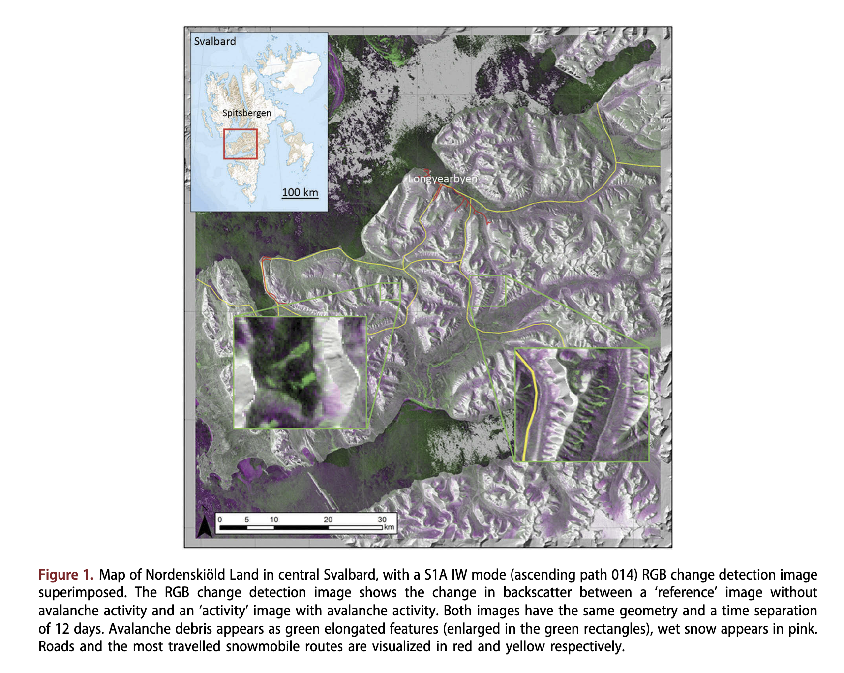
Nordenskiold Land is located in central Spitsbergen (Fig. 1), which is the largest island of the Svalbard Archipelago. Svalbard’s main settlement Longyearbyen (78°N, 15°E) is located in the northwestern corner of Nordenskiold Land, flanked by the IsHorden fjord. Mountain massifs intersected by wide valleys trending (north)east-(south)west dominate the landscape. These massifs are mostly comprised of flatlying sedimentary bedrock forming characteristic plateau-shaped mountains rising to a maximum height of ca. 1100 m asl and with an average altitude of ca. 420 m asl (Humlurn 2002). Typical winter weather is characterized by frequent low-pressure systems that bring warm air temperatures and heavy precipitation (Christiansen et al. 2013). These low-pressure systems transport warm and moist air to central Svalbard, resulting in large mid-winter air temperature fluctuations as well as mid-winter rain-on-snow events (Hansen et al. 2014). The majority of avalanche activity takes place during or directly after snowstorms induced by low-pressure activity and rain-on-snow events. Therefore the avalanche climate can be defined as a direct-action avalanche climate, according to Eckerstorfer & Christiansen (201 lb). These mid-winter rain-on-snow events result in extreme avalanche activity both in spatial distribution of avalanches as well as their sizes and run-outs (Eckerstorfer & Christiansen 2012). They also cause the snowpack to be thin and influence the snowpack structure, where ice layers and melt-forms acting as weak layers dominate (Eckerstorfer & Christiansen 2011a). The most common types of avalanches in Svalbard are slab avalanches, where a cohesive slab on top of a sliding surface or weak layer gets released (McClung & Schaerer 2011), and cornice-fall avalanches, where an overhanging mass of snow on ridge crests falls and triggers an avalanche (Vogel et al. 2012).
Data and methods
Satellite-borne SAR data
For this study, we use two different C-band SAR sensors on board the satellites SI A and RS2 (Table 1). SI A is part of the European Union’s Copernicus environmental monitoring programme, providing freely available SAR data from any point on Earth with a repeat cycle of 12 days. Because of Svalbard’s high latitude, SI A EW data (40 x 40 m2 spatial resolution) are available twice a day using different ascending and descending geometry paths, covering the Svalbard Archipelago entirely. Unfortunately, to date only one ascending path IW mode (15 x 25 m2 spatial resolution) is available from Svalbard, which we show in Fig. 1. RS2 is a commercial Canadian satellite that can provide on-order SAR data from any point on Earth. RS2 UF, with a spatial resolution of 3 x 3 m2 and a ground swath of 20 x 20 km2, can be ordered for free to a limited degree via a Norwegian quota.
Radar systems, such as those carried by S1A and RS2, can obtain images in different polarization modes. The transmitted and received waves can be either horizontal
to the slant range (horizontally polarized) or perpendicular to the slant range (vertically polarized). The polarization is indicated by two indices, where H stands for horizontal and V for vertically polarized. For this study, we obtained S1A images in co-polarization (HH) and cross-polarization (HV), whereas for RS2 only co-polarization (W) is used, as this was the only image available. Theoretically, cross-polarization is more sensitive to surface roughness, therefore better detectability of avalanche debris is expected.
The single most important factor for the detectability of avalanche debris is the sensors’ spatial resolution. According to Greene et al. (2010), avalanches of destructive force D2, which have a typical path length of 100 m, could bury, injure or kill a person. Such avalanche debris should therefore be detectable in RS2 UF images with 3 x 3 m2 spatial resolution. For avalanche debris to be detectable in S1A EW images with 40 x 40 m2 spatial resolution, the debris needs to be of nearly square or rectangular shape as opposed to a thin but elongated shape.
Manual identification and automatic detection of avalanche debris in SAR images
Step 0: SAR data pre-processing
The processing steps to arrive at automatic avalanche debris detection maps are listed below, and visualized in Fig. 2.
Earth ellipsoid model. The ground range detected high- resolution products were first calibrated using an annotated lookup table, before multi-looking was applied with 2x2 pixel averaging to suppress speckle. Using a DEM and precision orbit vectors, the radar coordinates were mapped to the selected UTM projection. The DEM was provided by the Norwegian Polar Institute in Tromso, Norway, and has a horizontal resolution of 20 m.
As a last step the backscatter products were projected to the output grid using the radar coordinate mapping as well as cubic interpolation. The output radar backscatter images oo(x, y) were stored as GeoTIFF files, with a corresponding radar shadow and layover mask, caused by radar geometry and the terrain, stored as a separate GeoTIFF file. We used the SAR processing software GSAR (Larsen et al. 2005) for geocoding and topographic correction pre-processing steps.
Step 1: create a slope angle mask
Based on the work of Buhler et al. (2013), the DEM (Step 0) was used to distinguish areas where avalanche debris could occur from areas where their occurrence was highly unlikely. This was done by masking out areas with slope angles <5° and >55° as the vast majority of stop avalanches occur on slopes with an angle between 25° and 55° (McClung & Schaerer 2011), however, their run-out zones extend to lower slope angles.
Step 2: create an RGB image
For manual identification of avalanche debris, we constructed enhanced RGB images that show the reference image in the red and blue channel, and the activity image in the green channel: [R, G, B] = [Ref image, Activity image, Ref image] (see example in Fig. 1). The reference image (aoref) was acquired 12 days before the activity image (aoavl) in case of all used S1A EW images. For the RS2 UF image, the reference image (aoref) was acquired after the activity image (aoavl), when the bare ground in the reference image posed a strong backscatter contrast to the activity image.

Step 3: manual identification of avalanche debris
Avalanche debris appears as green, tongue-shaped, downslope-stretching features in the RGB images from Step 2. The purpose of manual avalanche debris identification was to build up a validation data set that could be compared to the outputs of the automatic avalanche debris detection algorithm. Furthermore, we derived histograms of backscatter distribution of manually identified avalanche debris, which we used to arrive at backscatter thresholds that distinguish avalanche debris from undisturbed snow. We are aware that manual identification is subject to observer bias and difficult to reproduce. The identifications were carried out by an avalanche expert and controlled by a second researcher. We are confident to have manually identified all avalanche debris in the very high resolution RS2 UF image. The lower resolution of the S1A EW image created a challenge in identifying single avalanche debris when multiple avalanches occurred adjacent to each other.
Step 4: apply a median filter
An initial median filter with window size of 5 x 5 pixels was applied to the reference and avalanche images to reduce speckle.
Step 5: create a change detection image
We used a change detection method as basis for the automatic detection. This compiles a change detection image (Aao), which shows the backscatter difference between two temporally separated SAR images of similar geometry (Table 1):
Aao=aoavl-aoref,
where aoref and aoavl are the same reference and activity images as used for the manual identification method.
Step 6: apply the slope angle, layover and shadow mask
This step had the purpose to eliminate areas where avalanche debris either could not be detected (layover and shaded areas), as well as areas where the occurrence of avalanche debris was highly unlikely (slope angle mask). Both the topography as well as the incidence angle of the satellite determine how much terrain is affected by radar shadow and layover effects. In mountainous areas, radar shadow and layovers can affect up to 50% of avalanche terrain.
Step 7: apply thresholding
In this step, we determined a range of threshold values for distinguishing avalanche debris from undisturbed snow. The difference in backscatter coefficient inside and outside of the manually identified avalanche debris is visualized using histograms, where for the outside the mean backscatter of the image is taken, excluding the avalanche debris and the areas masked out (Step 6). The output of the thresholding was a binary image showing the pixels below and above the threshold value.
This backscatter thresholding, inspired by thresholding to detect wet snow by Nagler & Rott (2000), lies at the core of the automatic avalanche debris detection algorithm. Nagler & Rott (2000) used the decrease in backscatter from dry to wet snow conditions with a threshold of -3 dB. Here, we tested different thresholds of increasing backscatter, the results of which are shown below.
Step 8: apply filtering
After the thresholding, we applied a filter to smooth the results and eliminate noise. For the SI A EW mode data this post-classification filter was a self-designed RSO filter. The RSO filter connected areas with similar pixel values by testing for every pixel the eight neighbouring pixels. The output of the filter was the number of connected components and an array containing for every group of connected components the linear indices of the pixels in that group. This output was then used to eliminate all connected groups smaller or larger than the defined boundary, which is based on the minimum size of avalanche debris detectable in the SAR image and so adjusted to the image resolution.
Because of the very high resolution of the RS2 UF images, the RSO post-classification filter resulted in a large number of false detections. We therefore applied a simpler filter on this difference image, namely a median filter. This filter works by calculating for every pixel the median of the neighbouring pixels within a predefined window, in this case a window of 5 x 5 pixels. Although the resulting image looks slightly more blurred, the pixel spacing of the image is maintained.
Step 9: generate output
As an outcome of the automatic avalanche debris detection, we created maps showing the outlines of the detected avalanche debris. We used the publically available crowd-sourcing platform www.regObs.no maintained by the Norwegian Avalanche Centre to validate one of our SAR detected avalanche debris with field photographs.
Results
Manual identification of avalanche debris in S1AEW images
We manually identified avalanche debris in two RGB composites of ascending and descending geometry with an activity image from 18 March 2015 and a reference image from 6 March 2015. An example of the descending path RGB composite is shown in Fig. 3. The green elongated features were identified as avalanche debris and marked by white boxes. The identified avalanche activity is assumed to have been caused by a low-pressure system that brought air temperatures above freezing, as well as rain and high winds to Svalbard, starting 15 March 2015.
In total, seven unique avalanche debris were manually identified of which the avalanche in Fig. 3a was registered as a wet slab avalanche in www.regObs.no. The green tongue-shaped feature as observed in the RGB image corresponds well to the outline of the avalanche visible in the photograph (Fig. 3a). Wet avalanches have in general high surface roughness, which facilitates identification in SAR images. However, they are also often elongated in shape, which poses a problem in lower spatial resolution SAR images, where squared to rectangle shaped avalanche debris is more likely to be resolved.
In Table 2, we present the morphology of the avalanche debris and indicate whether they were identifiable in ascending and/or descending images with different polarization. Most identified avalanche debris occurred on north- to north-west- and west-facing slopes and were therefore more easily detected in the descending image that ‘looks’ to the left. All avalanche debris had lengths in the typical range of size 2.5-3 on the destructive force scale (Greene et al. 2010).
In general, avalanche debris exhibits higher backscatter than undisturbed snow (Fig. 4). This is especially true for the HV polarized images, where both populations are clearly distinguishable, overlapping only in the 0-5 dB range. The intersection between the histograms for oavi and oout is used for thresholding, distinguishing avalanche debris from undisturbed snow. For HV- polarized images the crossing lies between 3 dB and 4 dB, while for the НН-polarized images it lies around 2 dB. Cross-polarization (HV) is more sensitive to surface scattering, which is increased in rough avalanche debris, resulting in higher backscatter than under copolarization (HH).
Automatic avalanche debris detection in SI A EW images
We applied the automatic avalanche debris detection algorithm to the ascending and descending S1A EW images from 18 March 2015 in both polarization modes. In Fig. 5 we present the results for the HV polarized images which are more sensitive to surface roughness changes, applying threshold values of 3, 3.5 and 4 dB. By comparing the results of the automatic

Table 2. Summary statistics for manually identified avalanche debris in ascending and descending path S1A EW images with HV and HH polarization from 18 March 2015.
# | Aspect | Length (m) | Width (m) | Descending | Ascending | ||
HV | HH | HV | HH | ||||
1 | W | 270 | 240 | Y | N | N | N |
2 | NW | 300-570 | 180-190 | Y | Y | Y | Y |
3 | W | 670 | 180 | Y | Y | Y | Y |
4 | E | 390 | 200 | Y | N | Y | Y |
5 | NW | 650 | 120 | Y | Y | N | N |
6 | SE | 200-500 | 200-250 | Y | N | N | N |
7 | N | 290-480 | 120-230 | Y | Y | Y | Y |
Total Range |
| 200-670 | 120-250 | 7 | 4 | 4 | 4 |
detection with the manual identification we note that an increase in threshold leads to the algorithm missing a greater fraction of manually identified avalanche debris, but also to fewer non-identified avalanches which are likely to be false alarms. These statements hold true for all four images analysed (ascending/descending and НН/ HV) (Table 3). However, the descending activity image in HV polarization is the only image where 100% agreement was achieved, i.e., all identified avalanche debris were also automatically detected.
Manual identification of avalanche debris in RS2 UF images
We also show a second case study of avalanche debris detection using very high resolution RS2 UF data. The activity image is from 10 June 2013, with the reference image from 14 September 2013 (Fig. 6). The RGB image indicates wet snow (in pink) on the flat plateaus and in the majority of couloirs leading from the plateaus downslope. It also indicates snow-free conditions in the valley bottoms, shown in greyish green. The greyish green colour furthermore suggests that these low-lying areas have not experienced any major backscatter change between the activity and reference images.
We manually identified 13 avalanche debris in the ascending image, with the majority occurring on north-west- to north-east-facing slopes (Table 4). The avalanche debris were smaller than the ones detected in the S1A image. Not only does the very high resolution of the RS2 UF images allow for detection of small avalanche debris, it also allows to distinguish closely spaced avalanche debris adjacent to each other.
Also in this case, avalanche debris returns a higher backscatter signal than undisturbed snow (Fig. 7). The two peaks in this histogram denote the backscatter values from north-west- to north-east-facing slopes. Avalanche debris on north-west-facing slopes exhibits a higher backscatter coefficient than the ones on north-east-facing slopes because of the more favourable satellite imaging geometry and the local incidence angle. When we analysed the backscatter difference between the avalanche and reference image of three separate avalanche debris deposits, the intersection lay between 1.5 and 3 dB.
Automatic avalanche debris detection in RS2 UF images
Because of the very high resolution of the RS2 UF images, the RSO post-classification filter, applied to the SI A EW images, resulted in a lot of nonidentified avalanche debris. We therefore applied a simpler median filter with a window size of 5 x 5 pixels on the difference image before applying threshold values of 1.5, 2, 2.5 and 3 dB (Fig. 8). Again, the manually identified avalanche debris are encircled in red. The large black areas are glaciers (in the right upper corner and on the left), so we did not take them into account when determining the non-identified avalanches, as they can be clearly classified as not being avalanche debris. It would also be possible to create a mask to eliminate known glaciers before thresholding, as we may expect a distinct increase in backscatter for glaciers between June (wet snow cover) and September (likely exposed glacier ice) when the reference image was retrieved.


For a threshold value of 1.5 dB all manually identified avalanche debris were also automatically detected (Table 5), so again a 100% agreement was achieved. However, this detection method also resulted in a number of false positives. However, for higher threshold values this number decreases, but again at the expense of identified avalanches.
Table 3. Comparison of automatic avalanche debris detection and manual identification in descending and ascending and HV/HH polarized S1A EW images from 18 March 2015 using three different threshold values.
| Threshold (dB) | Agreement | ||
(-) | (%) | Non-identified | ||
(a) Descending - HV | 3 | 7 | 100 | >20 |
| 3.5 | 5 | 71 | 10 |
| 4 | 4 | 57 | 2 |
(b) Ascending - HV | 3 | 3 | 75 | 10 |
| 3.5 | 3 | 75 | 3 |
| 4 | 3 | 75 | - |
(c) Descending - HH | 2 | 6 | 86 | >20 |
| 2.5 | 4 | 57 | >20 |
| 3 | 3 | 43 | >10 |
(d) Ascending - HH | 2 | 3 | 75 | >20 |
| 2.5 | 3 | 75 | >20 |
| 3 | 2 | 50 | 9 |
Detectability of the extent of the avalanche debris
The very high resolution of the RS2 UF data has the advantage of capturing the tongue-shape outline of the avalanche in great detail. The zoomed-in view of the RS2 UF image in Fig. 9a shows three tongue-shaped features denoting avalanches and their debris extending northwards from a ridgeline. Comparing the same region in the automatically processed avalanche activity map, it becomes clear how well the area of the debris is captured (Figs. 9b-d). For higher thresholds, the automatic avalanche debris detection algorithm starts to miss debris closer to the starting zone, which is presumably because the snow has a lower surface roughness, causing less backscatter. This could cause an underestimation of the area damaged by the avalanche,
Table 4. Summary statistics for manual identified avalanche debris in the ascending path RS2 UF image with W polarization from 6 June 2013.
# | Aspect | Length (m) | Width (m) |
1 | NE | 400-450 | 40-50 |
2 | NE | 100-120 | 20-30 |
3 | NE | 140-250 | 10 |
4 | NW | 140-270 | 50-60 |
5 | NW | 120-130 | 50-60 |
6 | NW | 100-110 | 15-30 |
7 | NW | 100-180 | 15-40 |
8 | S | 270 | 35 |
9 | s | 235-240 | 25-35 |
10 | NW | 365-445 | 30-70 |
11 | NW | 240-255 | 55 |
12 | NW | 320-330 | 30-50 |
13 | NW | 120-190 | 30-50 |
Range |
| 100-450 | 10-70 |
and therefore an underestimation of its destructive potential. However, detection of the run-out zone seems to be less affected by higher thresholds because of its high surface roughness.
Discussion
Comparison of SI A EW and RS2 UF maps The three outstanding differences between S1A EW and RS2 UF images are their spatial resolution, their ground swath and their availability. The spatial resolution of RS2 UF images is 3 x 3 m2, which is significantly higher than the spatial resolution of 40 x 40 m2 for the S1A EW images. The difference in spatial resolution requires first and foremost different post-classification filters during the automatic avalanche debris detection. The S1A EW images require an RSO filter, whereas the RS2 UF images require a median filter. As for the manual identification and automatic detection of avalanche debris, the very high spatial resolution of RS2 UF images allows for the detection of small avalanche debris, that are in general harmless to people. However, it also allows for the detection of very thin, elongated avalanche debris of medium to large size that occur in ravines, couloirs and gullies. These avalanche debris can be a couple of hundreds of metres long but only a few

Table 5. Comparison of automatic avalanche debris detection and manual identification in the ascending path RS2 UF image with W polarization from 6 June 2013 using four different threshold values.
Agreement
Threshold (dB) | (-) | (%) | Non-identified |
1.5 | 13 | 100 | >50 |
2 | 12 | 92 | >50 |
2.5 | 10 | 77 | >50 |
3 | 8 | 62 | >50 |
metres wide, which the lower resolution S1A EW images cannot resolve. Thus, these types of avalanche debris that can pose a threat to life are not detected. The lower resolution of S1A EW images results also in the aggregation of multiple, adjacent avalanche debris into a single avalanche debris, leading to an underestimation in avalanche activity.
SI A EW images have a vastly larger ground swath of 400 x 400 km2 compared to RS2 UF’s 20 x 20 km2, potentially covering regional avalanche forecasting areas with a single image. With similar importance for operational use of SAR data in avalanche debris detection, SI A EW images can be acquired for free twice daily in Svalbard and every 12 days at any location on Earth. This allows for repeated production of change detection images and the collection of a complete data record in space and time. The disadvantage of a large ground swath is the varying degrees of radar incidence angle over the image, creating large radar shadow and layover effects in areas furthest away from the satellite, especially in mountainous topography. Areas affected by radar shadow and layover effects cannot be used for avalanche debris detection, which is certainly a problem in an operational context. This problem, however, can be easily overcome by using both ascending and descending path images over the same area. This way, all areas - except very narrow ravines and gullies - are illuminated by the radar and thus usable for avalanche detection.


Comparison between manual identification and automatic detection of avalanche debris
To quantify the performance of the automatic detection we used the results of the manual identification for comparison. Most of the manually identified avalanche debris were located on north-west-facing slopes, which is consistent with the general spatial pattern of avalanche activity in central Svalbard (Eckerstorfer & Christiansen 2011b). Prevailing south-easterly winds redistribute snow towards north-west-facing slopes, where avalanches frequently release. Nevertheless, manual avalanche identification is a subjective interpretation of SAR change detection images and therefore it is difficult to quantify the possible error in the identification. Avalanche debris exhibits a sharp change in backscatter between two SAR image acquisition dates. Eckerstorfer and Maines (2015) identified also active debris flow tracks, changing ice and snow conditions on glaciers and changing lake ice conditions as potential error sources. Using topographic maps and aerial photographs, these potential error sources can be eliminated. We are therefore confident that our manual identification method is trustworthy and can be used to evaluate the automatic avalanche debris detection algorithm. The largest error source we are aware of comes with the issue of pixel-to-pixel comparison between manual and automatic detection results (Vickers et al. in press). The exact manual delineation of avalanche debris deposit is difficult, especially in the uphill part of the deposit. Only the furthest run-out part of the avalanche debris deposit is in most cases bordered by a sharp backscatter contrast. Pixel resolution and local incidence angles complicate this issue further.
To find the optimal automatic detection method we want to maximize true positives and minimize false positives. Using a threshold of 3 dB resulted in 100% agreement between applying the manual and automatic detection method on the S1A data. However, over 20 sites were also detected by the automatic detection algorithm, but not manually identified as avalanche debris.
Applying the automatic avalanche debris detection algorithm to the very high resolution RS2 UF image with a threshold value of 1.5 dB resulted in 100% detectability of all 13 manually detected avalanche debris. Unfortunately, here also many areas were falsely detected, of which two were identified as glaciers.
Overall, we show that automatic detection of avalanche debris in both high and very high resolution C-band SAR images is possible. However, our algorithm needed to be adapted to the spatial resolution of the SAR images. Unfortunately, we did not have more SAR images with avalanche activity available for further testing of the algorithm. Obtaining a larger test sample would contribute significantly to fine- tuning the thresholding as well as post-processing, helping to eliminate the still high false positive rate. Moreover, by applying the automatic avalanche debris detection algorithm on consecutive images the activity of avalanches over time can be analysed. This can then be used as a condition in the automatic avalanche debris detection method to minimize the number of false alarms, e.g., pixels should be classified as avalanche debris only if they are detected in a set number of subsequent images.
Operational use of satellite-borne SAR detection of avalanche debris
Buhler et al. (2014) conducted a study to assess the technical feasibility and commercial viability of assisting avalanche forecasting in Europe by using supportive satellite data. In a user workshop, several gaps in avalanche forecasting were identified, of which the three most important ones were information on avalanche activity, snow surface conditions and snowpack stability. The users showed high willingness-to-pay for satellite data if they would provide highly reliable, daily updated high resolution information on avalanche activity. Currently, this is only achievable using terrestrial lidar (Prokop et al. 2008; Deems et al. 2015) or ground-based radar (Caduff, Schlunegger et al. 2015) systems, which are, however, only capable of monitoring a single slope (Eckerstorfer et al. 2016). Very high- resolution optical satellite data were recently used to detect avalanches with high true positives rates (Buhler et al. 2009; Lato et al. 2012). Buhler et al. (2009) suggests that the high number of false detections demands improvement of the algorithm before it can be implemented. Moreover, optical data are expensive, cover only comparably small areas and are weather- and light- dependent. However, the recent launch of the ESA Sentinel-2 satellite, with a spatial resolution of 10 m, repeatedly passing any location on Earth every 10 days might be a future possibility for operational use of optical satellite data in avalanche activity mapping.
Currently, however, space-borne radar satellite data are the most promising material for this task Radar satellite remote sensing does not suffer from weather and light dependency as the microwave signal can penetrate through clouds. As Svalbard experiences almost four months of polar night per year, radar is the only applicable technique for mapping avalanche activity. Likewise important for avalanche activity monitoring is both the spatial and temporal coverage of the satellite. The goal is ultimately to automatically process avalanche activity maps continuously throughout a winter. Besides the use of avalanche activity maps from SAR satellite data, we also envision that such data sets would be useful for geohazards mapping, communal planning, road closure and research into the effect of climate change on avalanche activity.
Both used SAR sensors are capable of detecting avalanche debris, however, both sensors have their limitations for operational use, which we discussed above. Lately, SI A started to acquire one image per repeat cycle in interferometric wide swath mode over Svalbard, with a higher spatial resolution of 15 x 25 m2 and a ground swath of 250 x 150 km2. With the launch of Sentinel-IB, hopefully more interferometric wide swath mode images will be taken of Svalbard, which would likely improve the detection of small to medium sized avalanche debris. The clear advantage of interferometric wide swath mode data for avalanche detection and the increasing need for improved avalanche monitoring in Nordenskiold Land indicate an even higher priority of interferometric wide swath mode over extra-wide swath mode in Svalbard, and we recommend that the ESA, particularly the Copernicus programme, reconsider their satellite acquisition policy.
Conclusion
We designed a method to automatically detect avalanche debris in SAR images. The automatic detection method is adapted to the available images and their spatial resolution. We applied the algorithm on medium resolution S1A EW images, and on very high resolution RS2 UF images.
We initially identified avalanche debris manually in change detection images of both sensors to (1) determine the backscatter threshold that best distinguishes avalanche debris from surrounding, undisturbed snow, and to (2) establish a data set to compare with the results of the automatic avalanche debris detection algorithm. By increasing the threshold value, the number of non-identified avalanche debris, likely to be false alarms, decreased along with the number of agreements. The automatic avalanche debris detection algorithm yielded better results in the S1A EW images than in the RS2 UF image. However, only large areas of avalanche debris were detectable in the S1A EW images and if two avalanche debris areas were in close proximity to each other they could be mistaken as one single area of avalanche debris. Nevertheless, S1A EW data have the advantage of being available twice a day for the whole of Svalbard, downloadable for free. With the availability of SIB data in autumn 2016 even more SAR data will be available, hopefully also in the higher resolution interferometric wide swath mode. This will allow for further improvement of our automatic detection method towards including the classification of pixels as avalanche debris only if they appear to be above the threshold value in
consequent images. We are confident that further testing and improvement of our developed automatic avalanche detection algorithm will lead to operational use of SAR avalanche detection in regional avalanche forecasting for Nordenskiold Land, Svalbard. These maps would be of great value for daily regional avalanche forecasting as complete and reliable information on avalanche activity is currently unavailable.
Acknowledgements
Radarsat-2 (RS-2) data were acquired under the Norwegian Radarsat-2 Agreement (MDA/NSC/KSAT, 2014 and 2015). Landsat-8 data were downloaded from http://earthexplorer.usgs.gov.Sentinel-1 data for 2014 and 2015 were downloaded from the European Space Agency Science Hub (https://scihub.esa.int/).
Disclosure statement
No potential conflict of interest was reported by the authors.
Funding
This research was conducted as part of the SeFaS project, financed by the Research Council of Norway and RDA Troms: Competence Centres in and for Northern Environments (contract no. TFK2013-248), a European Space Agency Living Planet Fellowship (AVISENT) and a project financed by the Norwegian Space Centre (JOP.07.16.2).
References
- Buhler Y., Bieler C., Pielmeier C., Wiesmann A., Caduff R., Frauenfelder R., Jaedicke C. & Bippus G. 2014. All- weather avalanche activity monitoring from space? In Proceedings, International Snow Science Workshop, Banff, 2014. Pp. 795-802. Bozeman, MT: International Snow Science Workshop/Montana State University Library.
- Buhler Y., Hum A., Christen M., Meister R. & Kellenberger T. 2009. Automated detection and mapping of avalanche deposits using airborne optical remote sensing data. Cold Regions Science and Technology 57, 99-106.
- Buhler Y., Kumar S., Veitinger J., Christen M., Stoffel A. & Snehmani. 2013. Automated identification of potential snow avalanche release areas based on digital elevation models. Natural Hazards and Earth System Sciences 13, 1321-1335.
- Caduff R., Schlunegger F., Kos A. & Wiesmann A. 2015. A review of terrestrial radar interferometry for measuring surface change in the geosciences. Earth Surface Processes and Landforms 40, 208-228.
- Caduff R., Wiesmann A., Buhler Y. & Pielmeier C. 2015. Continuous monitoring of snowpack displacement at high spatial and temporal resolution with terrestrial radar interferometry. Geophysical Research Letters 42, 813-820.
- Christiansen H.H., Humlum O. & Eckerstorfer M. 2013. Central Svalbard 2000-2011 meteorological dynamics and periglacial landscape response. Arctic, Antarctic, and Alpine Research 45, 6-18.
- Deems J.S., Gadomski J., Vellone D., Evanczyk R., LeWinter A., Birkeland K. & Finnegan D.C. 2015. Mapping starting zone snow depth with a ground- based lidar to assist avalanche control and forecasting. Cold Regions Science and Technology 120, 197-204.
- Eckerstorfer M., Buhler Y., Frauenfelder R. & Maines E. 2016. Remote sensing of snow avalanches: recent advances, potential, and limitations. Cold Regions Science and Technology 121, 126-140.
- Eckerstorfer M. & Christiansen H.H. 2011a. The “High Arctic maritime snow climate” in central Svalbard. Arctic, Antarctic, and Alpine Research 43, 11-21.
- Eckerstorfer M. & Christiansen H.H. 2011b. Topographical and meteorological control on snow avalanching in the Longyearbyen area, central Svalbard 2006-2009. Geomorphology 134, 186-196.
- Eckerstorfer M. & Christiansen H.H. 2012. Meteorology, topography and snowpack conditions causing two extreme mid-winter slush and wet slab avalanche periods in High Arctic maritime Svalbard. Permafrost and Periglacial Processes 23, 15-25.
- Eckerstorfer M. & Maines E. 2015. Manual detection of snow avalanche debris using high-resolution Radarsat-2 SAR images. Cold Regions Science and Technology 120,205-218.
- Greene E.M., Atkins D., Birkeland K.W., Elder K., Landry C., Lazar B., McCammon I., Moore M., Sharaf D., Sternenz B., Tremper B. & Williams K. 2010. Snow, weather, and avalanches: observational guidelines for avalanche programs in the United States. Pagosa Springs, CO: American Avalanche Association.
- Hansen B.B., Isaksen K., Benestad R.E., Kohler J., Pedersen A.0., Loe L.E., Coulson SJ., Larsen J.O. & Varpe 0. 2014. Warmer and wetter winters: characteristics and implications of an extreme weather event in the High Arctic. Environmental Research Letters 9, article no. 114021, doi: 10.1088/1748-9326/9/11/114021.
- Humlum O. 2002. Modelling late 20th-century precipitation in Nordenskiold Land, Svalbard, by geomorphic means. Norwegian Journal of Geography 56, 96-103.
- Larsen Y., Engen G., Lauknes T.R., Maines E. & Hogda K. A. 2005. A generic differential interferometric SAR processing system, with applications to land subsidence and snow-water equivalent retrieval. In Y. Larsen et al. (eds.): Proceedings of Fringe 2005 Workshop: 28 November-2 December 2005, Frascati, Italy. (CD-ROM.) P. 6. Noordwijk: ESA Publications Division.
- Lato MJ., Frauenfelder R. & Buhler Y. 2012. Automated detection of snow avalanche deposits: segmentation and classification of optical remote sensing imagery. Natural Hazards and Earth System Science 12, 2893-2906.
- Martinez-Vazques A. & Fortuny-Guasch J. 2007. Snow avalanche detection and classification algorithm for GB-SAR imagery. In: IEEE International Geoscience and Remote Sensing Symposium. IGARSS Barcelona 2007. Sensing and understanding our planet. Pp. 3740- 3743. Piscataway, NJ: IEEE Operations Center.
- McClung D. & Schaerer P. 2011. The avalanche handbook. Vol. 5. 3rd edn. Seattle: Mountaineers Books.
- McClung D.M. 2002. The elements of applied avalanche forecasting. Part II: the physical issues and the rules of applied avalanche forecasting. Natural Hazards 26, 131-146.
- Nagler T. & Rott H. 2000. Retrieval of wet snow by means of multitemporal SAR data. IEEE Transactions on Geoscience and Remote Sensing 38, 754-765.
- NGI (Norwegian Geotechnical Institute) 2017. Oppdatert ulykkesstatistikk. (Updated accident statistics.) Accessed on the internet at https://www.ngi.no/Tjenester/Fagekspertise-A-AA/Snoeskred/snoskred.no2/Ulykker-med-doed on 30 April 2017.
- Prokop A., Schirmer M., Rub M., Lehning M. & Stocker M. 2008. A comparison of measurement methods: terrestrial laser scanning, tachymetry and snow probing for the determination of the spatial snow-depth distribution on slopes. Annals of Glaciology 49, 210-216.
- Schweizer J. 2003. Rutschblock 73 - Verifikation der Lawinengefahr. (Rutschblock 73 - verification of the avalanche risk.) Bergundsteigen - Zeitschrift fur Risikomanagement itn Bergsport 12, 56-59.
- Schweizer J., Kronholm K. & Wiesinger T. 2003. Verification of regional snowpack stability and avalanche danger. Cold Regions Science and Technology 37, 277-288.
- Tedesco M. 2015. Remote sensing of the cryosphere. Oxford: Wiley-Blackwell.
- Ulaby F.T., Moore R.K. & Fung A.K. 1986. Microwave remote sensing: active and passive: from theory to applications. Pp. 1065-2162. Norwood, MA: Artech House.
- Vickers H., Eckerstorfer M., Maines E., Larsen Y. & Hindberg H. in press. Towards an automated snow avalanche debris detection method. Journal of Advances in Modeling Earth Systems.
- Vogel S., Eckerstorfer M. & Christiansen H.H. 2012. Cornice dynamics and meteorological control at Gruvefjellet, central Svalbard. The Cryosphere 6, 157- 171.
- Wiesmann A., Wegmueller U., Honikel M., Strozzi T. & Werner C.L. 2001. Potential and methodology of satellite based SAR for hazard mapping. In: Proceedings. IEEE 2001 International Geoscience and Remote Sensing Symposium. 9-13 July 2001. University of New South Wales, Sydney, Australia. Vol. 7. Pp. 3262-3264. Piscataway, NJ: IEEE Operations Center.