Satellite observations have shown a rapid decrease in sea ice in the Arctic Ocean. A number of factors have been put forward as the main causes of the reduction in sea ice in recent years: variations in the wind stress field and atmospheric warming (Köberle & Gerdes 2003; Rothrock & Zhang 2005; Stroeve et al. 2005); ice–albedo and ice–cloud feedback processes (Curry et al. 1995; Ikeda et al. 2003); an increase in heat transport from the Pacific Ocean to the Arctic Ocean through the Bering Strait (Woodgate et al. 2012); and an increase in Atlantic water heat transport to the Arctic Ocean (Zhang et al. 1998; Steele et al. 2008).

The retreat of summer sea ice in the Arctic Ocean continues to attract interest in exploring Arctic areas in order to locate and exploit natural resources and to establish shorter commercial shipping routes. Arctic sea routes (ASR) consist of two main paths: the North-eastern Passage, also called the Northern Sea Route (NSR), and the North-western Passage. The North-eastern Passage connects the Bering Strait and Kara Strait along the Russian Federation coastline. The North-western Passage cuts along the Alaskan coastline, the Canadian Archipelago and Baffin Bay. According to surveys (Schwarz 1995), the NSR can shorten the travel distance between the ports of Yokohama and Rotterdam by 40% compared to the existing southern sea route through the Suez Canal. Instead of one sole southern route, the existence of two routes would provide a tremendous boost for the security of international shipping.

In order to utilize the ASR, accurate sea-ice observations and predictions are vital to protect ships and offshore/coastal structures. Long-term, medium-term and short-term predictions are needed for safe navigation in the ASR. Long-term predictions—looking 20–30 years ahead—inform decisions regarding the construction of new icebreakers and ports. Medium-term predictions—about three to six months—contribute to decisions on whether to utilize the ASR or the conventional southern sea route in the coming summer navigation season. Finally, short-term predictions—one to two weeks—are used to choose the safest and shortest path in the Arctic Ocean once a ship enters ice-covered areas. This study considers how numerical modelling can be used to make short-term predictions of sea-ice conditions. Numerical modelling of sea ice has become an important instrument for ice monitoring, understanding past conditions, explaining recently observed changes and making future predictions regarding the Arctic Ocean.

The first collaborative research to examine the possibility of utilizing the NSR as an international commercial sea route was conducted from 1993 to 1999 by Japan, Norway and Russia when they advanced the International Northern Sea Route Programme (INSROP) (Kitagawa et al. 2001). INSROP has demonstrated the technical, ecological, environmental, economical, political and strategic aspects of the NSR. However, the INSROP project has not focused on developing a rigorous method of predicting sea ice along the NSR; sea-ice predictions have been dependent upon simple numerical predictions and satellite information.

In 1972–76, the Arctic Ice Dynamics Joint Experiment project advanced our understanding and modelling of sea-ice dynamics (Coon et al. 1974; Hibler 1979; Lu et al. 1989; Hopkins et al. 1991). Later, since 2001, the international Arctic Ocean Model Intercomparison Project (AOMIP) has focused on improving Arctic regional models and has investigated many aspects of the Arctic Ocean structure and sea-ice changes (Holloway et al. 2007). In general, most results obtained from the AOMIP numerical model accurately reproduce large-scale sea-ice dynamics using coarser resolution models. Meanwhile, some researchers (Leppäranta & Hibler 1985; Shen et al. 1986; Lu et al. 1989; Sagawa 2007) have focused on developing the theory of mesoscale sea-ice dynamics. In addition, some researchers have focused on reproducing and understanding Arctic Ocean structures. Wang et al. (2005) evaluated the seasonal cycle of sea-ice variables (ice volume and ice area) and ocean variables (heat and fresh water contents) in the pan-Arctic and North Atlantic Ocean using a coupled ice–ocean model with a 27.5 km resolution. Watanabe & Hasumi (2009) evaluated Pacific water transport across the Beaufort shelf break using an eddy-resolving coupled sea-ice–ocean model with a resolution of 2.5 km.

To date, there is no workable numerical model that is capable of resolving both mesoscale and large-scale sea-ice dynamics in the Arctic Ocean. Applications for making predictions for the ASR need a compromise model that will resolve complex sea-ice dynamics at both small and large scales. Almost all existing sea-ice forecast models are based on the continuum approach in ice dynamic processes. On a scale much larger than floe size (10–100 km), a continuum approximation is commonly assumed. Low computational cost and good description of large-scale sea-ice behaviour are the key attractions of continuum approximation. However, most of the available numerical models (Johnson et al. 2007; Johnson et al. 2012) have shown significant uncertainties in short-term and narrow-area predictions, especially for marginal ice zones.

In this study, we aim to reproduce the short-term sea-ice conditions in the ASR using a mesoscale eddy-resolving ice–ocean coupled model, while explicitly treating the ice discrete characteristics in marginal ice zones. Ice discrete characteristics are introduced to the model using Sagawa’s (2007) floe collision rheology. In addition, to minimize sea-ice diffusion and improve the accuracy of locating ice edges, we incorporate subgrid-scale ice motion (semi-Lagrangian movements) into the sea-ice dynamics (Rheem et al. 1997).

Model description

The ice–ocean coupled model developed in this study is based on a three-dimensional high-resolution regional model in the Sea of Okhotsk (Fujisaki et al. 2010) in which an ocean model is based on generalized coordinates, the Message Passing Interface version of the Princeton Ocean Model (POM; Mellor et al. 2002). The ice thermodynamics model is based on the zero-layer thermodynamic model proposed by Semtner (1976). The ice rheological model is based on the elastic–viscous–plastic (EVP) rheology proposed by Hunke & Dukowicz (1997) and Hunke (2001) and is modified to take ice floe collisions into account, following Sagawa & Yamaguchi (2006) and Sagawa (2007). The floe collision theory is based on the mixed discrete particle-continuum approach proposed by Rheem et al. (1997). Rheem’s formulation has proved to be very popular in coupled models because of its simplicity and explicit computation procedures. However, as Rheem’s formulation determines internal stress for all states of sea ice using the same formulas, which assume collision among rigid ice floes, the momentum propagation speed involved results in a marked increase in the explicit computation procedures. To overcome this numerical instability in explicit procedures, Sagawa & Yamaguchi (2006) and Sagawa (2007) introduced artificial compressibility into the sea-ice rheology. Ice strength parameter P is estimated following the empirical formulas derived by Sagawa & Yamaguchi (2006), Sagawa (2007) and Fujisaki et al. (2010):

To improve the ability of the ice–ocean coupled model (ice–POM) to locate ice edges, we implemented the Eulerian–Lagrangian method for advection (Rheem et al. 1997; Sagawa & Yamaguchi 2006) of the sea-ice variables (the so-called subgrid-scale ice motion). First, we solve the momentum equation in a Eulerian grid, and then we solve the ice conservation law in a Lagrangian grid. The ice field is represented by cylindrical floe particles (about 50 m in diameter) with a given thickness and bundle to the rectangular bunches. In each Eulerian grid cell, particles are summed for compactness and mean thickness, and then the momentum equation can be solved for velocities. Using the above Eulerian grid velocities, each Eulerian cell ice particle bunch is advected in space creating new configurations. Finally, a new ice state is obtained for the Eulerian grid by summing and redistributing the advected configurations.

The zonal and meridional grid spacings are approximately 25×25 km and 2.5×2.5 km for the whole-Arctic and high-resolution regional models, respectively. The vertical grid uses sigma coordinate systems with 33 levels for both models. To resolve the surface and bottom ocean dynamics, we use the logarithmic distribution of the vertical sigma layers near the top and bottom surfaces. To reduce the pressure gradient error (Haney 1991; Mellor et al. 1994) associated with sigma coordinates, the bottom topography is smoothed so that the bottom slope between two adjacent grid point ∣H₁∣−∣H₂∣/∣H₁∣+∣H₂∣≤0.175 (where H₁ and H₂ are the depths of the adjacent two grid points) is no greater than 0.175. The level-2.5 turbulence closure scheme of Mellor & Yamada (1982) is used for the vertical eddy viscosity and diffusivity. The horizontal eddy viscosity and diffusivity are calculated using a formula proportional to the horizontal grid size and velocity gradients (Smagorinsky 1963); the proportionality coefficient chosen is 0.2.

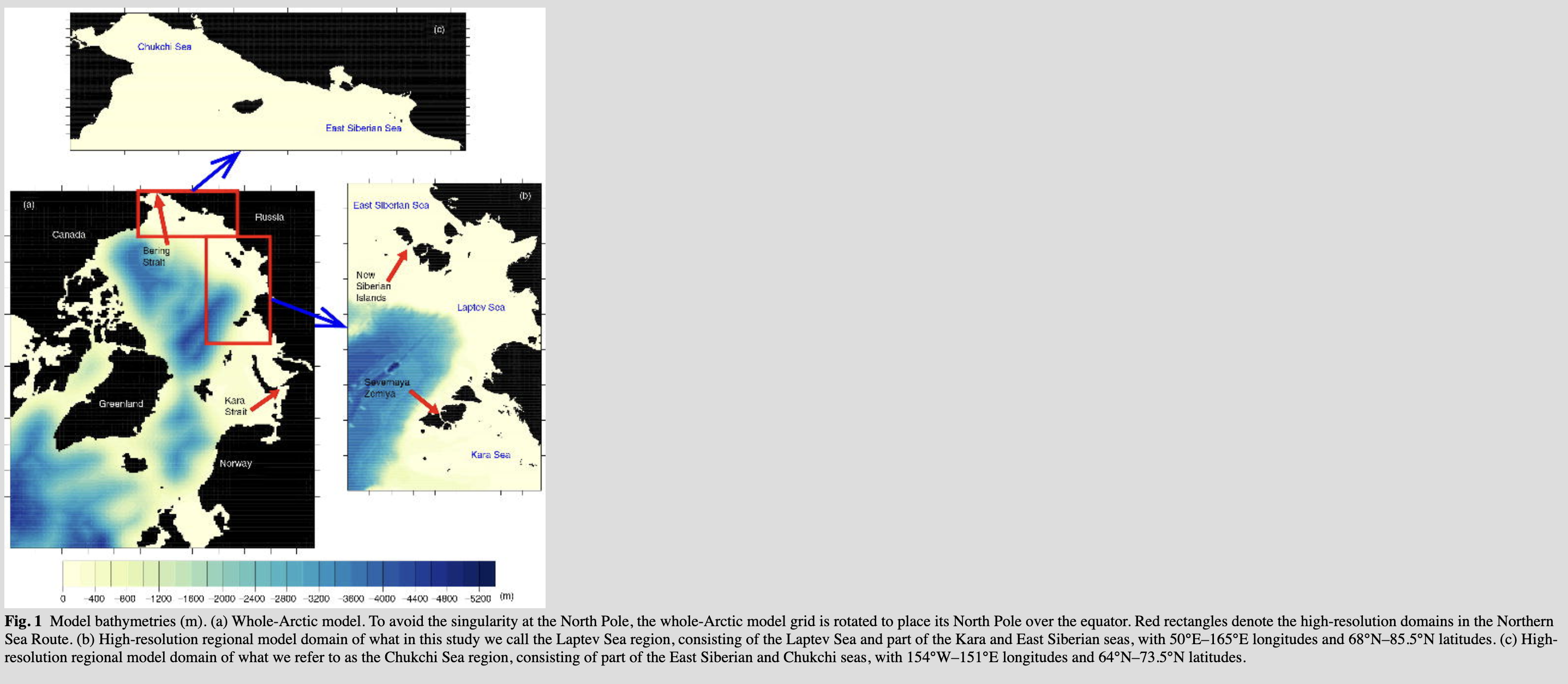
Figure 1 shows the model domains with a bottom topography based on the Earth Topography 1 Arc-minute Gridded Elevation Dataset (ETOPO1). What we call the Laptev Sea region (LS) includes the Laptev Sea and part of the Kara and East Siberian seas. What we call the Chukchi Sea region (CS) includes parts of the East Siberian and Chukchi seas.

The European Centre for Medium-Range Weather Forecasts Re-Analysis Interim (ERA-Interim) six-hourly data from 2000 to 2011 are given as the atmospheric forcing. Surface fluxes, shortwave radiation, longwave radiation, sensible heat flux and latent heat flux are calculated according to the bulk formulation proposed by Parkinson & Washington (1979). In the marginal regions of the whole-Arctic model, a radiation-boundary condition is applied for the ocean part, and an open-boundary condition is applied for the sea-ice part. In the marginal regions, salinity and temperature are relaxed to the monthly mean of the Polar Science Center Hydrographic Climatology (PHC3.0) data (Steele et al. 2001). In comparison, for the marginal regions of the high-resolution model, the whole-Arctic model results interpolated into high-resolution model grids are applied for both the sea-ice and ocean open-boundary conditions with daily intervals.

The sinusoidal seasonal cycles of the Bering Strait inflow are based on the observations of Woodgate et al. (2005) and the numerical experiments of Watanabe & Hasumi (2009). The inflow of the Pacific water in the Bering Strait is set to an annual mean of 0.8 Sverdrup (1 Sv=10⁶ m³ s⁻¹) and a seasonal amplitude of 0.4 Sv, with maximum inflow in June and minimum inflow in December. The salinity in the Bering Strait has an annual mean of 31 psu and a seasonal amplitude of 1 psu, with a maximum in March and a minimum in September. The temperature in the Bering Strait stays at the freezing point from January to June, and reaches its maximum value (5°C) in September. The 13 river water dischargers listed in the AOMIP website (www.whoi.edu/page.do?pid=30587) are prescribed as the surface freshwater flux at each river mouth.

The whole-Arctic model time integration started without specifying the initial sea-ice and ocean currents, and only specifying the climatological temperature and salinity fields provided by PHC3.0. First, the model was spun up for 15 years by providing atmospheric data for the year 2000 cyclically. The total sea-ice volume in the entire model domain reached an equilibrium state after the 15-year spin up. Then the model was integrated from 2000 to 2011 with ERA-Interim atmospheric forcing.

Numerical instability in a high-resolution ice–POM model

The ice–POM model has been used to study sea-ice behaviour in the Sea of Okhotsk (Fujisaki et al. 2010) for several years. Ice–POM simulations have provided better information on sea-ice behaviour and on ice-edge locations than other basic models (Watanabe et al. 2004) as a result of the ice collision rheological formulation and subgrid-scale ice motions. However, when we applied the ice–POM model to the Arctic Ocean, undesirable and fatal numerical instabilities occurred near coastal regions. This numerical instability is initiated once the wind field tries to push the sea ice toward the coastline. As a result of these numerical instabilities, sometimes the ice–POM model crashed because of a Courant–Friedrichs–Lewy condition violation, or generating unphysical values in ice thickness and ice velocities. As previously mentioned, Sea of Okhotsk simulations did not show this unphysical behaviour in the older version of the ice–POM model (Fujisaki et al. 2010). A number of reasons could account for this strange behaviour of Arctic simulations, the most dominant of which is that the average wind field in the Sea of Okhotsk is not against the coastlines, unlike the case for the Arctic Ocean. Another reason could be the underlying warm ocean structure in the Sea of Okhotsk area, which accelerates ice melting before the propagation of numerical instabilities.

Lipscomb et al. (2007) described similar numerical instability issues using a one-dimensional benchmark test set-up, as shown in Supplementary Fig. S1. They explained the instability results as being due to unstable communication between the ridging scheme and the dynamics, which is caused by the abnormal increment of ice strength within a short time period. Their numerical model is significantly different from the ice–POM model because they use multiple ice-thickness categories and adopt ridging schemes and strength parameterization based on Rothrock (1975) and Thorndike et al. (1975). But in the ice–POM model, we use a single thickness category and ice collision strength parameterization.

To explain the numerical instabilities in the ice–POM model, we repeat the one-dimensional benchmark test analysis of Lipscomb et al. (2007). Consider a one-dimensional domain similar to that shown in Supplementary Fig. S1. The wind is specified to blow from west to east with no variation in the y direction. The east and west boundaries are closed and land boundary conditions are used. The north and south boundaries are open, and open- and periodic-boundary conditions are used. The domain is initialized with a motionless uniform sea-ice thickness of 2.73 m at an 80% concentration. Thermodynamics variation of sea ice, Coriolis force and sea-surface tilt force are not considered in this one-dimensional test problem.

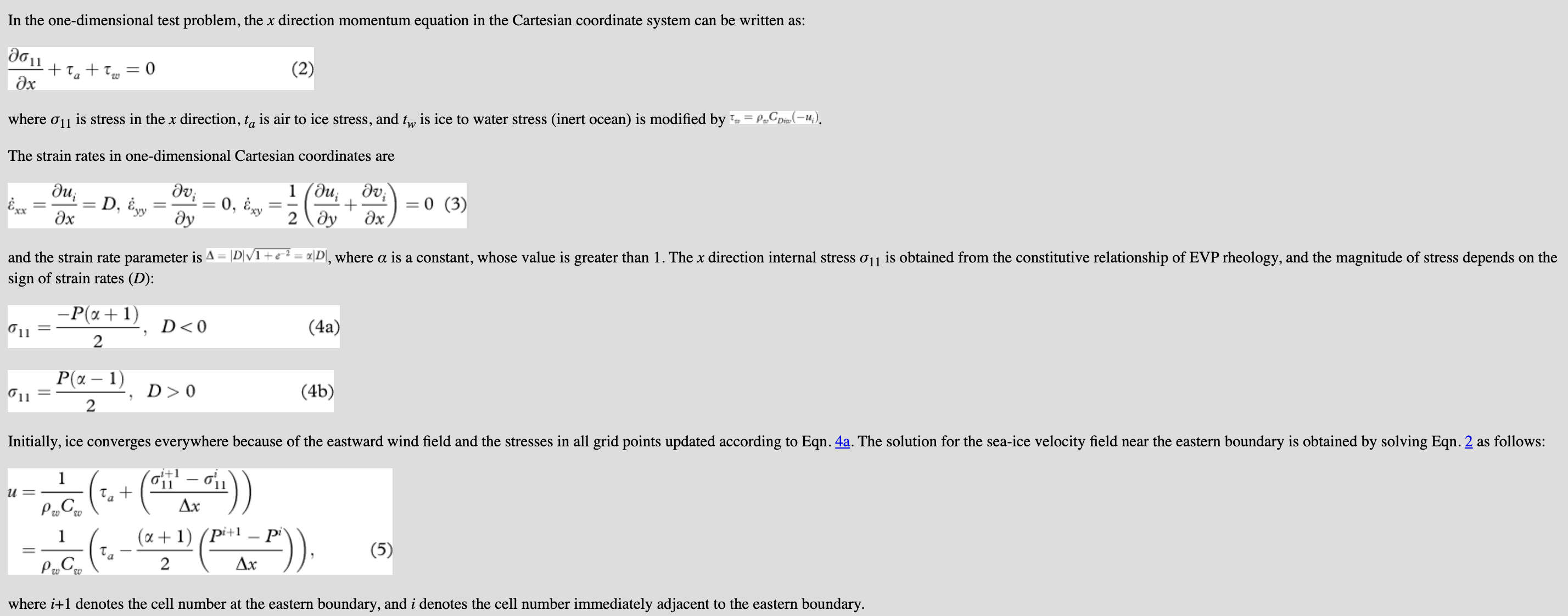
In the earlier formulation, the ice strength in collision rheology is determined by Eqn. 1. Figure 2 shows the variation in the sea-ice strength of the collision rheology formulation and the standard EVP rheology formulation with respect to the sea-ice concentration and strain rate parameters. If the ice concentrations are nearly 100%, then ice strength P can increase significantly whatever the strain rates in our collision rheology formulation. As ice internal stresses are functions of P, the solution for ice velocity loses its accuracy because of the sudden increment of P. Consider in a given time step, the ice strength at east boundary Pⁱ⁺¹ overshoots and the stress gradient (Pⁱ⁺¹–Pⁱ)/Δx exceeds the wind stress. According to Eqn. 5, ice flow should be reversed in the grid cell near the east boundary (i+1). If the ice flow reverses, the divergence (D) is positive in grid cell i+1 and the solution for momentum equation changes near the eastern boundary grid as follows. Note that the upstream grid cells are converging (D<0) because of the eastward wind.

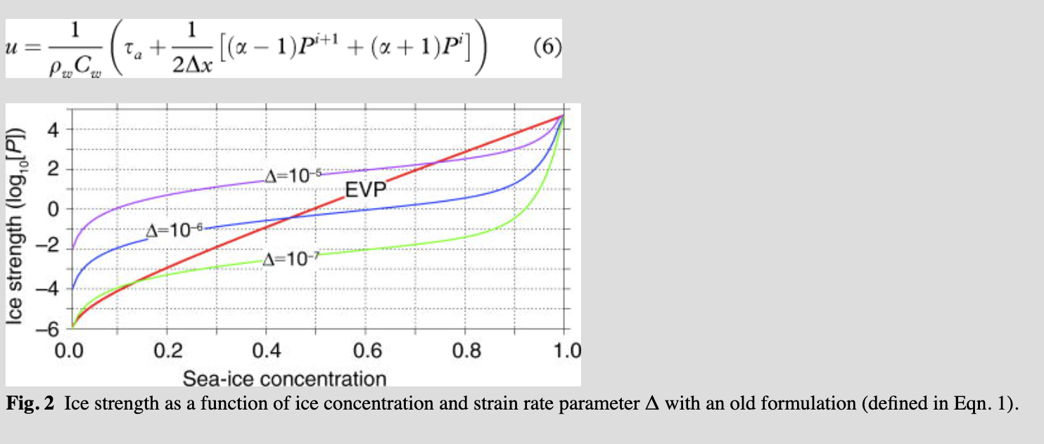
However in the next time step, the velocity should be positive (because α>0 and Pⁱ⁺¹>Pⁱ>0) in the grid cell at eastern boundary, as the right-hand side of Eqn. 6 is positive. Therefore, the ice flow field becomes converged again and the velocities are given in Eqn. 8. The magnitude of P is not changed during this process, and the strength gradient supports the wind stress and therefore the ice flow must be reversed. If this process continues, the ice flow field starts oscillating near the solid boundaries and neighbouring grid cells. If the numbers of EVP cycles are large enough (small time steps), the oscillations damp down and are restored toward a true solution. Otherwise, the oscillations are amplified and the model produces an unphysical thick ice and oscillating flow fields.

This instability issue is fundamentally numerical and is triggered by the sudden increment of ice strength at the 100% concentration. In the real physical process of floe collision, however, Sagawa (2007) and Shen et al. (1986) showed that floe collision becomes maximum at the ice concentration equivalent with maximum compactness (A_max approximately 90% concentration). In our old formulation, ice floes collided frequently at a 100% concentration. In light of this, we changed the old collision rheology formulation of Eqn. 1 to adopt the maximum floe collision concentration to (A_max) 90% as follows:

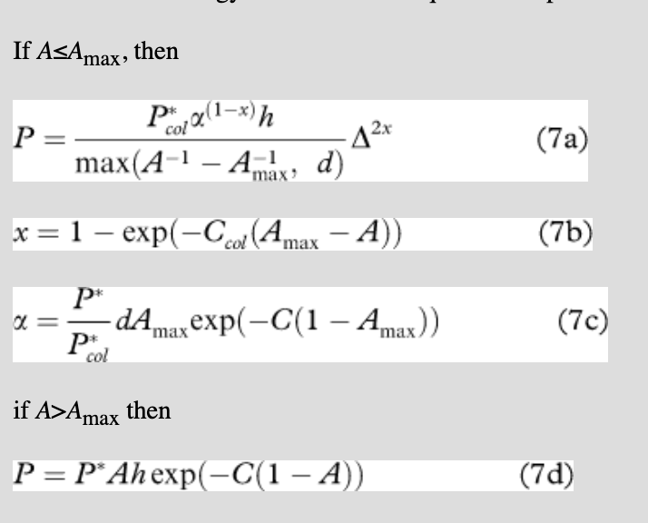
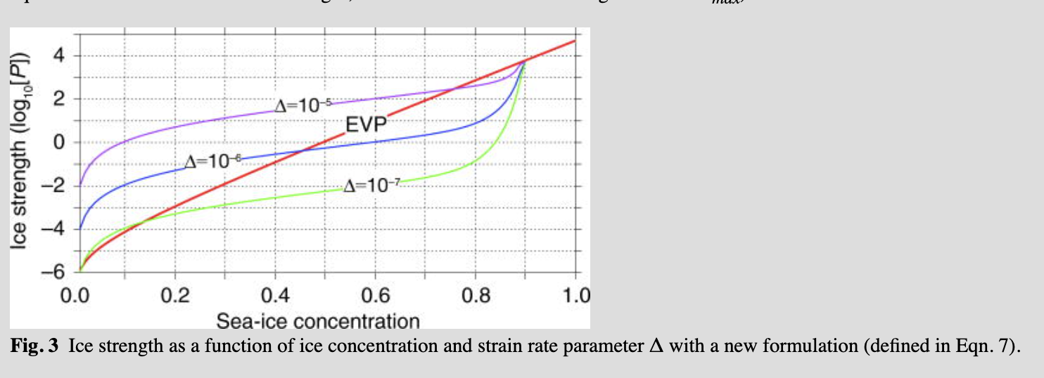
Equation 7 changes the ice strength P with respect to the ice strain rates and ice concentrations as shown in Fig. 3. This physically realistic modification allows the ice strength to relax when concentrations are greater than 90% (ice strength P is equal to the EVP formulation ice strength, when the ice concentration is greater than A_max).

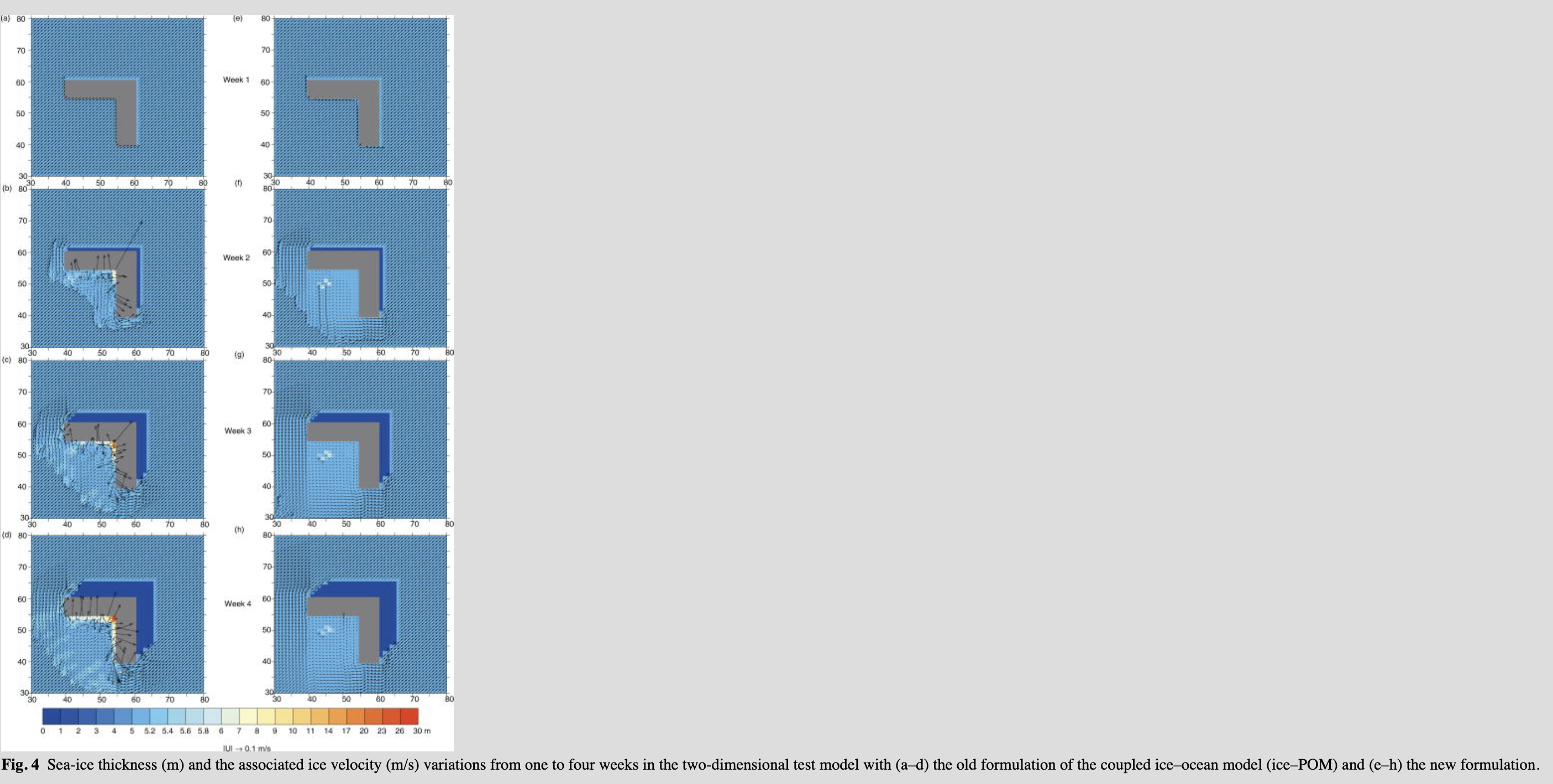
To make a comparison of the new modifications of collision rheology, we have considered the two-dimensional problem [as did Lipscomb et al. (2007)] with a domain similar to that shown in Supplementary Fig. S2. All the boundaries of the two-dimensional domain are open, and periodic- and open-boundary conditions are used. In the middle of the domain there is an L-shaped island. The domain is initialized with motionless sea ice with a uniform thickness of 5 m and a concentration of 80%. The wind is specified to blow from the south-west to the north-east at a speed of 14.1 m/s. Thermodynamic variations of sea ice, the Coriolis force and sea-surface tilt force are not considered, even in the two-dimensional test problem.

Figure 4a–d shows the ice thickness and associated velocity field near the L-shaped island for the old formulation. After the first week, an unstable ice flow develops upwind of the island where the ice pack converges. Instabilities soon spread over a large region and produced thick sea ice and a noisy velocity field near the L-shaped island. In comparison, the sea ice converged nicely and the ice flow field was damped throughout the computation period in the new modified version (Fig. 4e–h).

Whole-Arctic model reproducibility

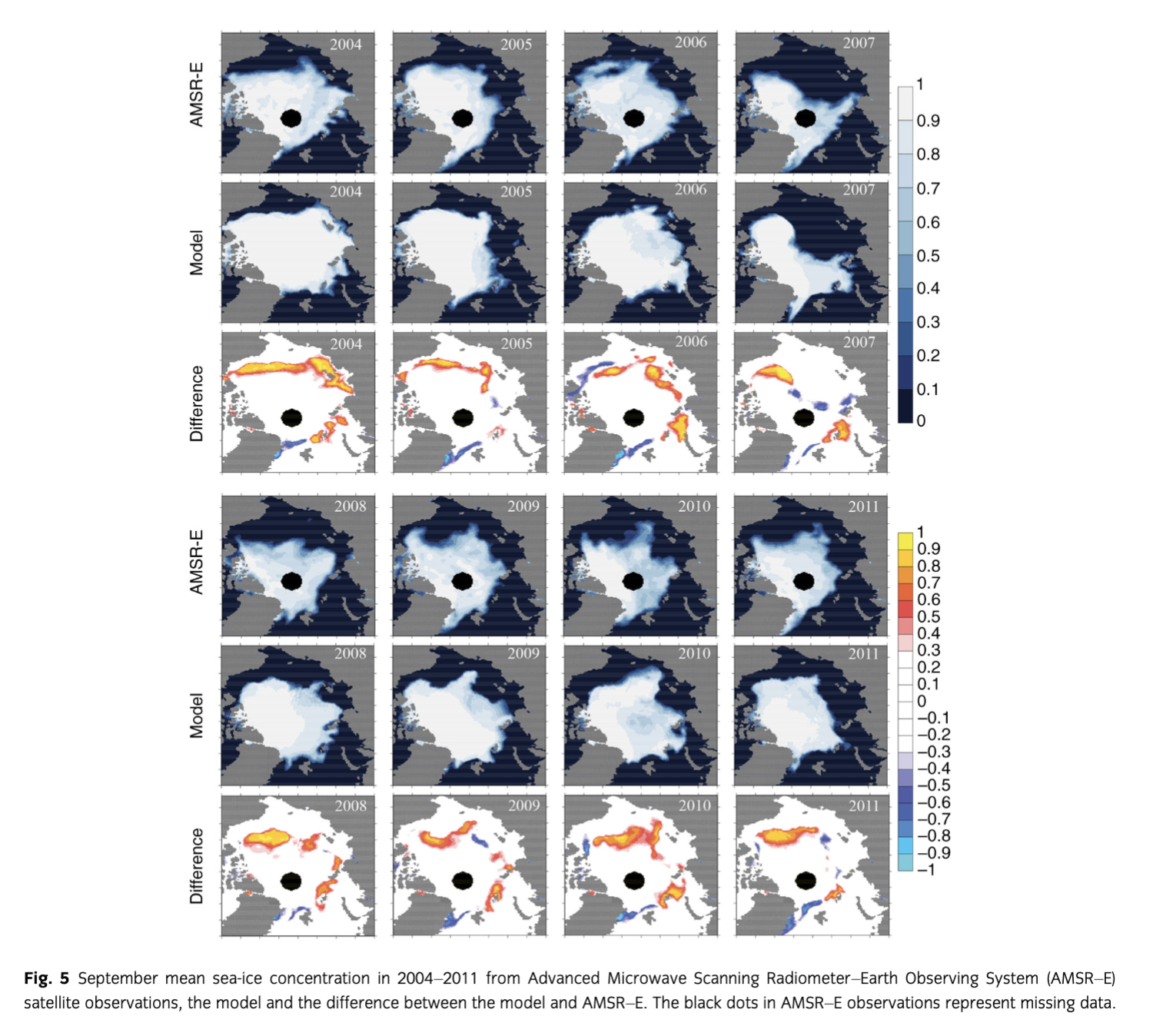
In this section, we examine the reproducibility of the model in detail. To assess how well the ice–POM simulates the concentration, extent, thickness and motion of sea ice, we use several satellite-derived products and in situ observational data. Sea-ice concentration is one of the most important of the sea-ice properties that have to be reproduced faithfully, and is the only property for which many reliable observations are available to validate numerical models. Figure 5 shows the mean sea-ice concentration of the model for September compared with observational sea-ice concentrations for corresponding months obtained from the Advanced Microwave Scanning Radiometer–Earth Observing System (AMSR–E) data set, and the difference between the model and the AMSR–E concentrations. The model captured the negative trend in the September Arctic sea-ice extent, the year 2007 minimum sea-ice extent and the year 2005 opening of the North-eastern Passage. In September, the AMSR–E data show that the Alaskan coast and the Russian coast are free of ice and that the ice concentration in the Canadian Archipelago is reduced. This spatial distribution pattern is captured by the ice–POM model (Fig. 5 shows the difference between the model and the AMSR–E concentrations). In general, the ice–POM model overestimates the sea-ice concentration around the Canadian Basin. We believe that the overestimation of the ice concentration in the Canadian Basin in the ice–POM is due to the poor mesoscale eddy-resolving capability in the coarser resolution (25 km) whole-Arctic simulation. This is because mesoscale eddies play a significant role in distributing summer Pacific water into the Canadian Basin (Watanabe & Hasumi 2009).

To understand the reproducibility of the interannual behaviour of the ice–POM sea ice, we analysed the sea-ice extents from 2001 to 2011. The observational data were obtained from the data set provided by Cavalieri et al. (1996). This data set is provided with a polar stereographic grid, which makes a direct comparison difficult with the ice–POM numerical model. To overcome this, observational data are interpolated into the 25-km resolution whole-Arctic model grid. Also for the comparison, we disregarded grid cells that have concentrations of less than 15%. Figure 6 shows comparisons of the daily sea-ice extent with satellite observations. The model captures the major features of observed sea-ice concentration properties, including minimum sea-ice extents for the years 2007 and 2011. The correlation coefficient between the model and observations is 0.98; the model slightly underestimates the sea-ice extent in summer. We believe that the discrepancy between the model and the observational sea-ice extents is due to the simplified thermodynamics in this ice–POM model (especially the constant albedo values, sea ice 0.7, snow 0.9 and seawater 0.1, and the disregarding of melt ponds), and the lack of reproducibility of multi-year thick ice.

Next we focus on the ability of the ice–POM model to reproduce sea-ice thickness as compared to the observations. The observational sea-ice thickness data used in this study were obtained from the new Unified Sea Ice Thickness Climate Data Record (Lindsay 2010). There are currently more than 3000 samples available for access in this data set. The observational thickness data are derived from various observational methods, including the Ice, Cloud, and Land Elevation Satellite (ICESat), airborne electromagnetic, moorings and submarines and drill holes.

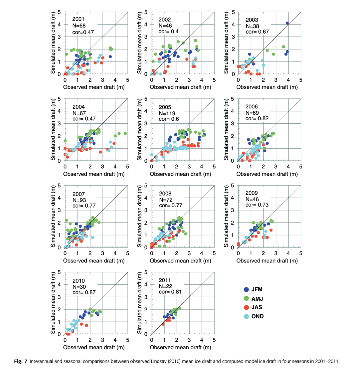
A scatter diagram between the modelled and observed thickness from 2001 to 2011 is shown in Fig. 7. The differences between the model and observational thickness data are significant in winter and spring, with correlation coefficients of 0.54 and 0.52, respectively. On the other hand, in summer and autumn, the correlation between the modelled and observed thicknesses is reasonable, with 0.74 and 0.61 correlation coefficients, respectively. It can also be seen that our model captures thin ice (<2 m) and underestimates thick ice (>2 m). We believe that one of the main reasons for the underestimation of thick ice in the ice–POM model is the lack of thickness categories in our model (we used mean thickness). The mean-thickness approach is a very crude system in which information on actual ice thickness can easily disappear; that said, this assumption simplifies the models. However, in thickness-category models, sea-ice thickness is represented using the thickness distribution of Thorndike et al. (1975). With this method, it is possible to include thickness variability in the numerical models. Furthermore, looking at the correlation coefficients in Fig. 7, we can clearly see that our model reproduced the observational sea-ice thickness after the year 2007 reasonably well, on account of the disappearance of thick ice in the Arctic Ocean after the year 2007 minimum sea-ice record.

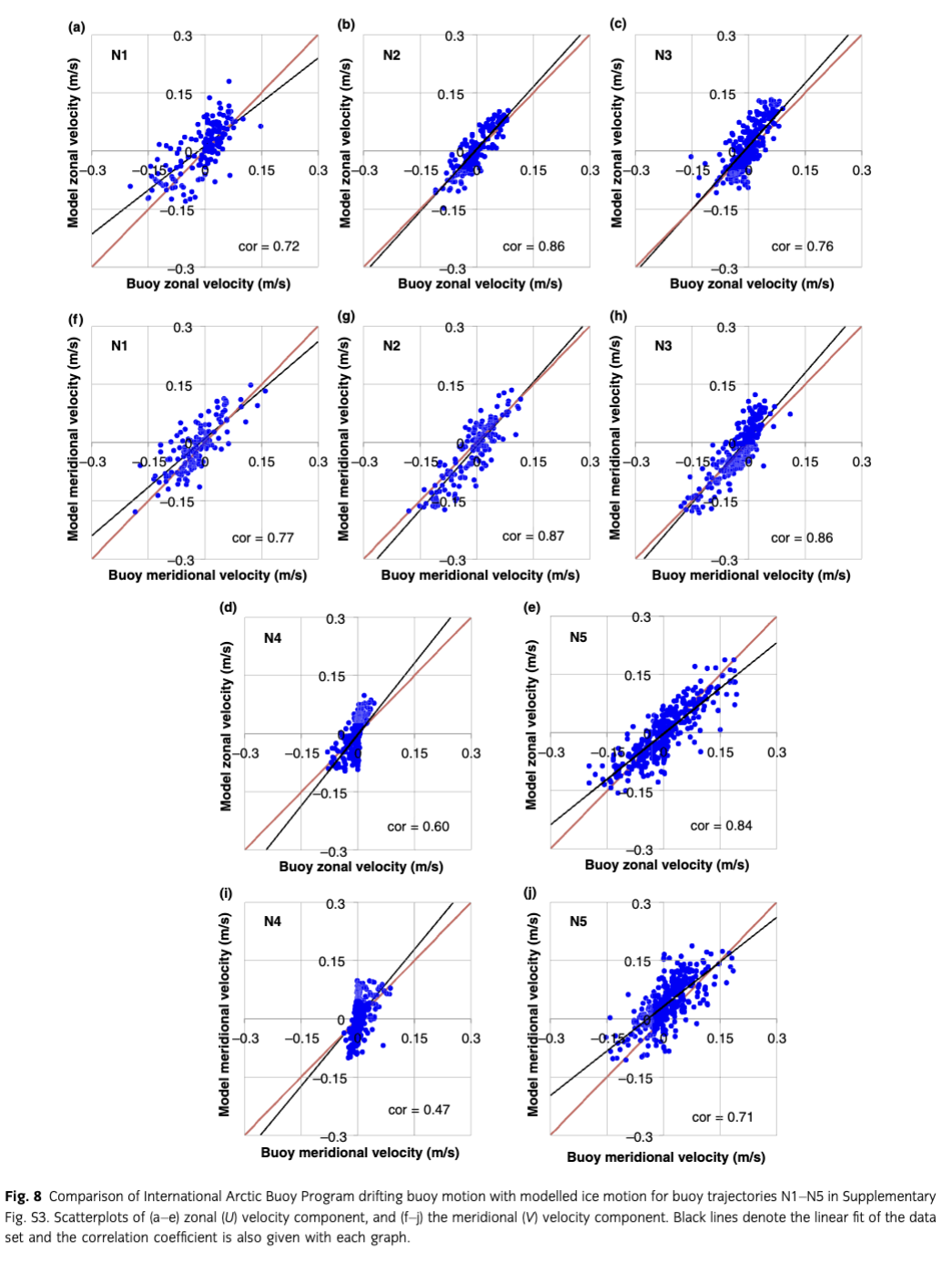
Finally, we compared the model-derived ice velocity with data on buoy positions obtained from the International Arctic Buoy Program. We found that the formation of leads, ridges and polynyas were mainly caused by movement of the sea ice. In addition, we found that the position of the ice edge, which depends on a supply of sea ice from the interior ice pack, is greatly influenced by ice motion. Because the position of the ice edge is crucial information for safe navigation in the ASR, ice drift is an important variable that needs to be reproduced correctly in sea-ice modelling. Here, we compare and analyse model-derived and observed sea-ice velocities.

Supplementary Fig. S3 shows buoy trajectories from International Arctic Buoy Program from 1 January 2004 to 31 December 2004. For this comparison, the ice–POM model ice velocities at each buoy position (Supplementary Fig. S3) are evaluated using the weighted average Gaussian interpolation method.

A comparison of buoys and model velocities from 1 January 2004 to 31 December 2004 shows a high correlation coefficient in both velocity components (Fig. 8). However, the correlation coefficients vary with the initial buoy locations and show a minimum correlation (0.47) near the Canadian Archipelago (N4), where the ice thickness in our model and in the observations shows the maximum difference. The model shows the best correlation coefficients of 0.87 in the transpolar drift areas (N2) and near the Fram Strait areas (N3), because our model reproduces the ice thickness to some extent in both the regions. It should be noted that the model–data comparison is made without considering uncertainties in the buoy data.

High-resolution hindcast simulation along the NSR

As shown above, the whole-Arctic model was able to capture sea-ice conditions accurately. However, we describe below how the whole-Arctic coarser resolution model cannot be used to accurately predict the details of ice-edge locations and extents. For safe navigation in the ASR, we need to investigate the sea-ice variables in a more detailed manner. To analyse the details of sea-ice dynamics and to carry out accurate ice predictions in the North-eastern Passage of the ASR, we chose two main regions for high-resolution modelling (Fig. 1). Comparison of the model results with observations and the importance of high-resolution computations are discussed in this section.

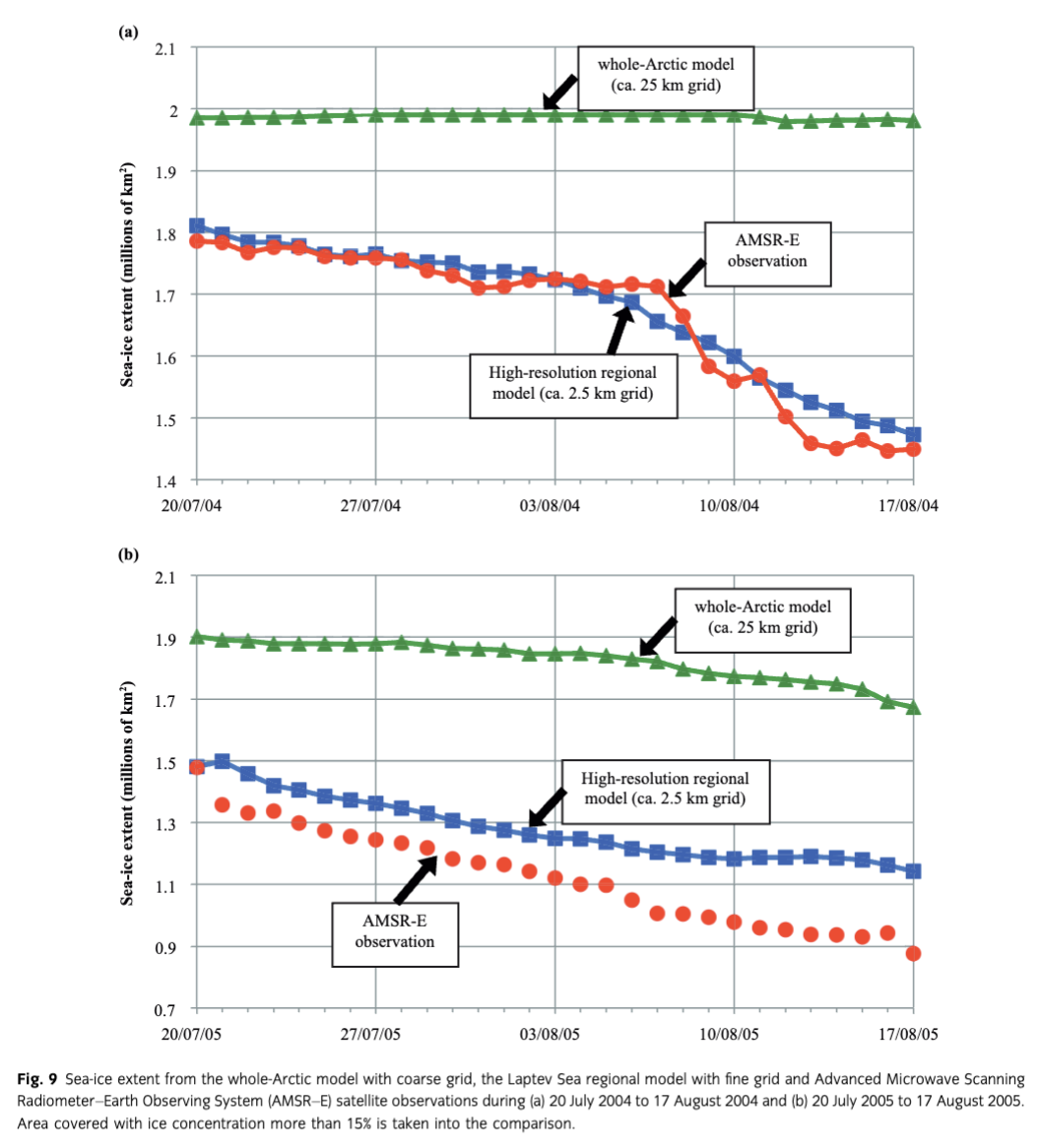
Figures 9 and 10 show a time series of sea-ice extent in the LS and CS regions for short-term (four-week) hindcast simulations in 2004 and 2005, respectively. These two years were chosen because the North-east Passage was closed in 2004, whereas 2005 was a year in which it was open. High-resolution computations are initialized using interpolated whole-Arctic model results (e.g., sea-ice thickness, ocean temperature and salinity). Note that whole-Arctic sea-ice concentration is not used for high-resolution computations; rather, satellite observations (AMSR–E) are used. When the initial AMSR–E sea-ice concentration is not zero in the open water area of the whole-Arctic simulation, we interpolated the sea-ice thickness from neighbouring grid cells. In this case, water surface temperature under those cells was set to freezing temperature to avoid the rapid melting of sea ice. Moreover, when the initial AMSR–E observed concentration is zero and the whole-Arctic simulation concentration is not zero, we set the sea-ice thickness to zero in those cells. For those cells, the temperature under the ocean surface was assigned by interpolating the values only from the open water neighbouring grid cells. Note that, in both situations, ocean salinity is unchanged and the same as the interpolated whole-Arctic model output value.

In the marginal regions (open boundaries) of the high-resolution model, the whole-Arctic model results interpolated into the high-resolution model grids are applied for both the sea-ice and ocean open-boundary conditions with daily intervals.

In both the LS and CS regions, computations are performed from 20 July to 17 August in the years 2004 and 2005. As shown in Fig. 9a, the sea-ice extent simulated in the LS regional model varied from 1.8×10⁶ km² to 1.4×10⁶ km² within the four-week period in 2004 because of thermodynamics and dynamics activities. In the first two weeks, the computation shows a similar reduction pattern with observations. In the third week, the observational sea-ice extents show a dramatic reduction, but the model cannot capture such a dramatic reduction. At the end of the third week (11 August 2004), the model sea-ice extent is almost equal to the observational results. But again in the fourth week, the model has drifted away from the observation. Figure 9b shows the model sea-ice extent variation from 1.5×10⁶ km² to 1.1×10⁶ km² in 2005. In contrast to 2004, when the North-east Passage was closed, the high-resolution regional model overestimates the sea-ice extent compared to the observations in the opening year of 2005. Instead of high-resolution computations, the coarse-grid whole-Arctic computation (extracted LS region) cannot reproduce the ice-extent variations in both years. Sea ice in the whole-Arctic model was almost unchanged in 2004, while it showed a slightly decreasing trend throughout the 2005 computations.

As shown in Fig. 10, the sea-ice extent in 2004 and 2005 varied in the CS region from 0.5×10⁶ km² to 0.05×10⁶ km² within the four weeks. However, the difference between the observations and the model is much larger (about 0.1×10⁶ km²) in 2004 than in 2005. In contrast to the LS region, the whole-Arctic simulation (extracted CS region) showed a similar decreasing trend in sea-ice extent compared to satellite observations in the CS region.

In addition to the quantitative comparisons of sea-ice extent, we compared the sea-ice concentration qualitatively. Figure 11 shows the LS region model concentration and the AMSR–E satellite observed concentration (Cavalieri et al. 2014) and difference between the model and AMSR–E sea-ice concentrations over the period 20 July to 17 August 2004. Note that AMSR–E passive microwave sensors cannot distinguish melt ponds from open water and they therefore underestimate sea-ice concentration when melt ponds are present; such uncertainties are not taken into account for this comparison. For the first two weeks, the difference in sea-ice concentration is low compared to the last two weeks. On the west side of the New Siberian Islands (Fig. 11), it can be seen that the model somewhat overestimates the concentrations. We believe this discrepancy could be due to the uncertainties in the model initial conditions. This is because we used sea-ice thickness data from the interpolated whole-Arctic model for our high-resolution computations as an initial condition. The south-west part of the regional model and observational data show similar concentration variations and ice-edge locations. PHC3.0 climatological observational data show that this area has a higher sea-surface temperature in the summer. Therefore, this south-west part of the region of the ice boundary is most likely controlled by the thermodynamics process rather than the ice dynamic process.

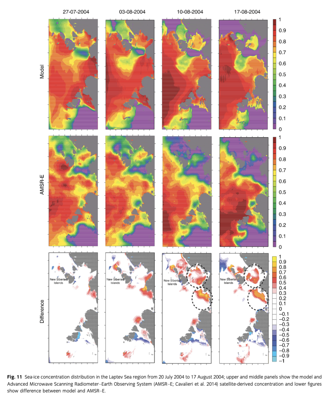
Considering all the qualitative and quantitative comparisons of the regional model results, we believe that the coarse-grid computation cannot be used to reproduce sea-ice variations in summer accurately. But the fine-grid computation can reproduce sea-ice variations accurately using satellite observations. However, even high-resolution computations are unable to follow the dramatic reduction of sea-ice extents, as shown in Fig. 9a.

There are several possible reasons for this discrepancy in the results between coarser and high-resolution grid computations. The first reason is mesoscale eddy-resolving capability. Johannessen et al. (1987) and Li et al. (2013) discussed the important of ice–eddy interaction process in the Arctic Ocean. As shown in Fig. 12, the high-resolution computation reproduces the mesoscale eddies for a 20–50 km radius in the ocean, whereas the coarser resolution whole-Arctic computation cannot reproduce the mesoscale eddies. The mesoscale eddies in the ocean draw out ice from the main body and move to the slightly warmer water areas, which enhances melting. Melted ice supplies low-salinity cold water to the ocean surface and activates the production of eddies due to baroclinic instability. In addition, the correct representation of mesoscale eddies and surface ocean current help to correct the momentum transfer of the ice–ocean interface. The detailed mechanisms of mesoscale eddy generations are discussed elsewhere.

The second possible reason is that small-scale sea-ice dynamics (converging and diverging process) were more correctly captured with the high-resolution models than with the coarser grid models. The local converging and diverging process is mainly influenced by ocean current and wind. If the ocean current or wind pushes the ice together, the ice extent is reduced. We call this the converging process. If the ocean current or wind spread out the ice, the ice extent is increased. We call this the diverging process. Correctly resolving small- and large-scale converging and diverging processes of sea-ice in high-resolution models improved the sea-ice edge locations (Fujisaki et al. 2007) and ice extents significantly.

The third possible reason is that the high-resolution computation well expresses the ice-albedo feedback process, which accelerates ice melting in the spring and summer. In the current model, snow, sea ice and seawater have different constant albedo values. The total albedo of a given grid cell depends on the area covered with sea ice and open water.

Conclusion

New shipping routes in the Arctic Ocean will require the accurate prediction of sea-ice conditions. In this study, we used a high-resolution ice–ocean coupled model that uses ice collision rheology to predict sea-ice conditions in the marginal ice zones on timescales of one to two weeks.

We showed that abrupt changes in the ice strength P (due to the floe collision rheology used in the earlier version of the model) can cause instability in the high-resolution ice–POM sea-ice model. The symptoms of the instability are noisy and unrealistic sea-ice thickness, ice concentration, strength, velocity and strain rates. An unstable flow typically arises near islands and coastlines where convergence and shear are large. Modification of floe collision near maximum compactness (about 90% concentration) and a new method of proper damping of elastics waves in EVP rheology successfully resolved the instability issues in the ice–POM model without a need to reduce the time step interval.

We investigated the reproducibility of basic features in the ice–POM model using the coarser resolution (about 25 km) whole-Arctic model. The model reproduced the seasonal and interannual variations in sea-ice extents, thickness and Arctic sea-ice circulations reasonably well. In comparison, the coarser resolution whole-Arctic ice–POM model cannot be used to reproduce the correct fresh water transport and accumulation in the Arctic Ocean (not shown in this paper). Many researchers (e.g., Watanabe & Hasumi 2009) have suggested that Pacific water is transported into the Canada Basin by mesoscale eddy activities, which are barely resolved in coarser resolution models. In our next paper, we are planning to discuss the mesoscale eddies and sea-ice interaction quantitatively. Even although the whole-Arctic model well reproduced the overall trends of the Arctic sea ice, it cannot be used to predict the sea ice in the short term. However, the high-resolution regional model reproduced the short-term and narrow-area sea-ice extents and concentrations found in the observational data.

In terms of accurately forecasting sea ice using a high-resolution ice–ocean coupled model, appropriate initial conditions and realistic forcing data must be input. The incorporation of data assimilation techniques into the whole-Arctic numerical model may improve the initial conditions of high-resolution models. At this point, the lack of observational sea-ice data and the coarseness of the reanalysis forcing data are key impediments to accurate forecasts and validating model results in the Arctic. Despite those limitations, our findings show that this model can be used to predict short-term sea ice accurately.

Acknowledgements

The authors wish to acknowledge support from the Green Network of Excellence Program Arctic Climate Change Research Project by the Japanese Ministry of Education, Culture, Sports, Science and Technology and a Kakenhi grant (no. 26249133) from the Japan Society for the Promotion of Science. Their gratitude is extended to Professors Hiroyasu Hasumi, Daisuke Kitazawa, Kozo Sato and Chang-kyu Rheem for their advice during the progress of this study. The authors also thank the anonymous reviewers for their valuable comments and advice.

References

1. Cavalieri D.J., Markus T. & Comiso J.C. 2014. AMSR–E/Aqua Daily L3 12.5 km brightness temperature, sea ice concentration, & snow depth polar grids, Version 3. Boulder, CO: National Aeronautics and Space Administration Distributed Active Archive Center at the National Snow and Ice Data Center.


2. Cavalieri D.J., Parkinson C.L., Gloersen P. & Zwally H. 1996. Sea ice concentrations from Nimbus–7 SMMR and DMSP SSM/I–SSMIS passive microwave data. Boulder, CO: National Aeronautics and Space Administration Distributed Active Archive Center at the National Snow and Ice Data Center.


3. Coon M.D., Maykut G.A., Pritchard R.S., Rothrock D.A. & Thorndike A.S. 1974. Modeling the pack ice as an elastic–plastic material. AIDJEX Bulletin 24, 1–105.


4. Curry J.A., Schramm J.L. & Ebert E.E. 1995. Sea ice–albedo climate feedback mechanism. Journal of Climate 8, 240–247. Publisher Full Text


5. Fujisaki A., Yamaguchi H., Duan F. & Sagawa G. 2007. Improvement of short-term sea ice forecast in the southern Okhotsk Sea. Journal of Oceanography 63, 775–790. Publisher Full Text


6. Fujisaki A., Yamaguchi H. & Mitsudera H. 2010. Numerical experiments of air–ice drag coefficient and its impact on ice–ocean coupled system in the Sea of Okhotsk. Ocean Dynamics 60, 377–394. Publisher Full Text


7. Haney R.L. 1991. On the pressure gradient force over steep topography in sigma coordinate ocean models. Journal of Physical Oceanography 21, 610–619. Publisher Full Text


8. Hibler W.D. III. 1979. A dynamic thermodynamic sea ice model. Journal of Physical Oceanography 9, 815–846. Publisher Full Text


9. Holloway G., Dupont F., Golubeva E., Häkkinen S., Hunke E., Jin M., Karcher M., Kauker F., Maltrud M., Morales Maqueda M.A., Maslowski W., Platov G., Stark D., Steele M., Suzuki T., Wang J. & Zhang J. 2007. Water properties and circulation in Arctic Ocean models. Journal of Geophysical Research—Oceans 112, C04S03, doi: http://dx.doi.org/10.1029/2006JC003642


10. Hopkins M.A., Hibler W.D. III & Flato G.M. 1991. On the numerical simulation of the sea ice ridging process. Journal of Geophysical Research—Oceans 96, 4809–4820. Publisher Full Text


11. Hunke E.C. 2001. Viscous–plastic sea ice dynamics with the EVP model: linearization issues. Journal of Computational Physics 170, 18–38. Publisher Full Text


12. Hunke E.C. & Dukowicz J.K. 1997. An elastic–viscous–plastic model for sea ice dynamics. Journal of Physical Oceanography 27, 1849–1867. Publisher Full Text


13. Ikeda M., Wang J. & Makshtas A. 2003. Importance of clouds to the decaying trend and decadal variability in the Arctic ice cover. Journal of the Meteorological Society of Japan 81, 179–189. Publisher Full Text


14. Johannessen J.A., Johannessen O.M., Svendsen E., Shuchman R., Manley T., Campbell W.J., Josberger E.G., Sandven S., Gascard J.C., Olaussen T., Davidson K. & Van Leer J. 1987. Mesoscale eddies in the Fram Strait marginal ice zone during the 1983 and 1984 marginal ice zone experiments. Journal of Geophysical Research—Oceans 92, 6754–6772. Publisher Full Text


15. Johnson M., Gaffigan S., Hunke E. & Gerdes R. 2007. A comparison of Arctic Ocean sea ice concentration among the coordinated AOMIP model experiments. Journal of Geophysical Research—Oceans 112, C04S11, doi: http://dx.doi.org/10.1029/2006JC003690


16. Johnson M., Proshutinsky A., Aksenov Y., Nguyen A.T., Lindsay R., Haas C., Zhan J., Diansky N., Kwok R., Maslowski W., Häkkinen S., Ashik I. & de Cuevas B. 2012. Evaluation of Arctic sea ice thickness simulated by Arctic Ocean Model Intercomparison Project models. Journal of Geophysical Research—Oceans 117, C00D13, doi: http://dx.doi.org/10.1029/2011JC007257


17. Kitagawa H., Ono N., Yamaguchi H., Izumiyama K. & Kamesaki K. 2001. Northern sea route. Shortest sea route linking East Asia and Europe. Tokyo: Ship & Ocean Foundation.


18. Köberle C. & Gerdes R. 2003. Mechanisms determining the variability of Arctic sea ice conditions and export. Journal of Climate 16, 2843–2858. Publisher Full Text


19. Leppäranta M. & Hibler W.D. III 1985. The role of plastic ice interaction in marginal ice zone dynamics. Journal of Geophysical Research—Oceans 90, 11899–11909. Publisher Full Text


20. Li Q., Zhang Z. & Wu H. 2013. Interaction of an anticyclonic eddy with sea ice in the western Arctic Ocean: an eddy-resolving model study. Acta Oceanologica Sinica 32, 54–62. Publisher Full Text


21. Lindsay R.W. 2010. Unified sea ice thickness climate data record. Available from the Polar Science Center, Applied Physics Laboratory, University of Washington at psc.apl.washington.edu/sea_ice_cdr


22. Lipscomb W.H., Hunke E.C., Maslowski W. & Jakacki J. 2007. Ridging, strength, and stability in high-resolution sea ice models. Journal of Geophysical Research—Oceans 112, C03S91, doi: http://dx.doi.org/10.1029/2005JC003355


23. Lu Q., Larsen J. & Tryde P. 1989. On the role of ice interaction due to floe collisions in marginal ice zone dynamics. Journal of Geophysical Research—Oceans 94, 14525–14537. Publisher Full Text


24. Mellor G.L., Ezer T. & Oey L.-Y. 1994. The pressure gradient conundrum of sigma coordinate ocean models. Journal of Atmospheric and Oceanic Technology 11, 1126–1134. Publisher Full Text


25. Mellor G.L., Hakkinen S., Ezer T. & Patchen R. 2002. A generalization of a sigma coordinate ocean model and an intercomparison of model vertical grids. In N. Pinardi & J. Woods (eds.): Ocean forecasting: conceptual basis and applications. Pp. 55–72. Berlin: Springer.


26. Mellor G.L. & Yamada T. 1982. Development of a turbulence closure model for geophysical fluid problems. Reviews of Geophysics 20, 851–875. Publisher Full Text


27. Parkinson C.L. & Washington W.M. 1979. A large-scale numerical model of sea ice. Journal of Geophysical Research—Oceans and Atmospheres 84, 311–337. Publisher Full Text


28. Rheem C.K., Yamaguchi H. & Kato H. 1997. Distributed mass/discrete floe model for pack ice rheology computation. Journal of Marine Science and Technology 2, 101–121. Publisher Full Text


29. Rothrock D.A. 1975. The energetics of the plastic deformation of pack ice by ridging. Journal of Geophysical Research—Oceans and Atmospheres 80, 4514–4519. Publisher Full Text


30. Rothrock D.A. & Zhang J. 2005. Arctic Ocean sea ice volume: what explains its recent depletion? Journal of Geophysical Research—Oceans 110, C01002, doi: http://dx.doi.org/10.1029/2004JC002282


31. Sagawa G. 2007. Development of ice dynamic model that takes account of floe collision and its validation in numerical sea ice forecast in the Sea of Okhotsk. (In Japanese.) PhD thesis, University of Tokyo.


32. Sagawa G. & Yamaguchi H. 2006. A semi-Lagrangian sea ice model for high resolution simulation. In J.S. Chung (ed.): Proceedings of the Sixteenth International Offshore and Polar Engineering Conference. Pp. 584–590. Cupertino, CA: International Society of Offshore and Polar Engineers.


33. Schwarz J. 1995. Can the Northern Sea Route be profitable. In H. Kitagawa (ed.): Northern Sea Route; future and perspective. Proceedings of the INSROP Symposium Tokyo ’95. Pp. 605–614. Tokyo: Ship and Ocean Foundation.


34. Semtner A.J. 1976. A model for the thermodynamic growth of sea ice in numerical investigations of climate. Journal of Physical Oceanography 6, 379–389. Publisher Full Text


35. Shen H.H., Hibler W.D. III & Leppäranta M. 1986. On applying granular flow theory to a deforming broken ice field. Acta Mechanica 63, 143–160. Publisher Full Text


36. Smagorinsky J. 1963. General circulation experiments with the primitive equations. Monthly Weather Review 91, 99–164. Publisher Full Text


37. Steele M., Ermold W. & Zhang J. 2008. Arctic Ocean surface warming trends over the past 100 years. Geophysical Research Letters 35, L02614, doi: http://dx.doi.org/10.1029/2007GL031651 Publisher Full Text


38. Steele M., Morley R. & Ermold W. 2001. PHC: a global ocean hydrography with a high-quality Arctic Ocean. Journal of Climate 14, 2079–2087. Publisher Full Text


39. Stroeve J.C., Serreze M.C., Fetterer F., Arbetter T., Meier W., Maslanik J. & Knowles K. 2005. Tracking the Arctic’s shrinking ice cover: another extreme September minimum in 2004. Geophysical Research Letters 32, L04501, doi: http://dx.doi.org/10.1029/2004GL021810 Publisher Full Text


40. Thorndike A.S., Rothrock D.A., Maykut G.A. & Colony R. 1975. The thickness distribution of sea ice. Journal of Geophysical Research—Oceans and Atmospheres 80, 4501–4513. Publisher Full Text


41. Wang J., Liu Q., Jin M., Ikeda M. & Saucier F.J. 2005. A coupled ice-ocean model in the pan-Arctic and North Atlantic Ocean: simulation of seasonal cycles. Journal of Oceanography 61, 213–233. Publisher Full Text


42. Watanabe E. & Hasumi H. 2009. Pacific water transport in the western Arctic Ocean simulated by an eddy-resolving coupled sea ice–ocean model. Journal of Physical Oceanography 39, 2194–2211. Publisher Full Text


43. Watanabe T., Ikeda M. & Wakatsuchi M. 2004. Thermohaline effects of the seasonal sea ice cover in the Sea of Okhotsk. Journal of Geophysical Research—Oceans 109, C09S02, doi: http://dx.doi.org/10.1029/2003JC001905


44. Woodgate R.A., Aagaard K. & Weingartner T.J. 2005. Monthly temperature, salinity, and transport variability of the Bering Strait through flow. Geophysical Research Letters 32, L04601, doi: http://dx.doi.org/10.1029/2004GL021880


45. Woodgate R.A., Weingartner T.J. & Lindsay R. 2012. Observed increases in Bering Strait oceanic fluxes from the Pacific to the Arctic from 2001 to 2011 and their impacts on the Arctic Ocean water column. Geophysical Research Letters 39, L24603, doi: http://dx.doi.org/10.1029/2012GL054092 Publisher Full Text


46. Zhang J., Rothrock D.A. & Steele M. 1998. Warming of the Arctic Ocean by a strengthened Atlantic inflow: model results. Geophysical Research Letters 25, 1745–1748. Publisher Full Text