This article is published under a Creative Commons license and not by the author of the article. So if you find any inaccuracies, you can correct them by updating the article.

The number and distribution of polar bears in the western Barents Sea


Jon Aars
Tiago A. Marques
Karen Lone
Magnus Andersen
Øystein Wiig
Ida Marie Bardalen Fløystad
Snorre B. Hagen
Stephen T. Buckland
Published: Oct. 9, 2017
Latest article update: Aug. 9, 2023
This article is published under the license


Abstract
Polar bears have experienced a rapid loss of sea-ice habitat in the Barents Sea. Monitoring this subpopulation focuses on the effects on polar bear demography. In August 2015, we conducted a survey in the Norwegian Arctic to estimate polar bear numbers and reveal population substructure. DNA profiles from biopsy samples and ear tags identified on photographs revealed that about half of the bears in Svalbard, compared to only 4.5% in the pack ice north of the archipelago, were recognized recaptures. The recaptured bears had originally been marked in Svalbard, mostly in spring. The existence of a local Svalbard stock, and another ecotype of bears using the pack ice in autumn with low likelihood of visiting Svalbard, support separate population size estimation for the two areas. Mainly by aerial survey line transect distance sampling methods, we estimated that 264 (95% CI = 199 – 363) bears were in Svalbard, close to 241 bears estimated for August 2004. The pack ice area had an estimated 709 bears (95% CI = 334 – 1026). The pack ice and the total (Svalbard + pack ice, 973 bears, 95% CI = 334 – 1026) both had higher estimates compared to August 2004 (444 and 685 bears, respectively), but the increase was not significant. There is no evidence that the fast reduction of sea-ice habitat in the area has yet led to a reduction in population size. The carrying capacity is likely reduced significantly, but recovery from earlier depletion up to 1973 may still be ongoing.
Keywords
Svalbard, Ursus maritimus, helicopter, habitat loss, sea ice, distance sampling
Polar bears (Ursus maritimus) live in Arctic areas with sea ice as their main habitat (Amstrup 2003). Their preferred prey are sea-ice-associated seal species (Amstrup 2003). Polar bears also depend on sea ice to travel between mating, breeding and feeding sites (Stirling & Derocher 2012). The total population size is assumed to be about 20 000 - 25 000 polar bears distributed in 19 subpopulations in Canada, Greenland, Norway, Russia and the USA (Obbard et al. 2010). However, both subpopulation size and trend are unknown for several of these subpopulations. Unsustainable hunting was formerly supposed to be the only considerable threat to the polar bears leading to the signing of The Agreement on the Conservation of Polar Bears in 1973 (Prestrud & Stirling 1994). As a result of this agreement, polar bears were totally protected in Norwegian areas in 1973 (Ekker et al. 2013). Today, habitat loss due to a warming Arctic and melting sea ice is the main concern for the persistence of polar bears (Stirling & Derocher 2012; Wiig et al. 2015; Regehr et al. 2016). Polar bears have been identified as one of the marine mammal species most vulnerable to a warming climate and sea-ice habitat loss in the Arctic (Laidre et al. 2008).
The Barents Sea polar bears have experienced the fastest loss of sea-ice habitat of all the 19 recognized subpopulations in the Arctic, with an increase in the duration of the summer season (from spring sea-ice retreat to fall sea-ice advance) by about 20 weeks during the period 1979-2013 (Laidre et al. 2015; Stern & Laidre 2016). It is also predicted that the Barents Sea polar bears will experience a more profound loss of habitat in the next decades compared to most other subpopulations (Durner et al. 2009; Laidre et al. 2015).

The rapid loss of sea-ice habitat in the Arctic may have lowered the polar bear carrying capacity well below historical levels, and is expected to drop further as the habitat is predicted to continue to shrink (Durner et al. 2009; Laidre et al. 2015; Wiig et al. 2015; Regehr et al. 2016; Stern & Laidre 2016). The size of the Barents Sea polar bear subpopulation was estimated to be between 1900 and 3600 bears in August 2004 (Aars et al. 2009). It was further concluded that the subpopulation likely must have been much larger historically to sustain an average annual take of about 300 bears over a century (Lons 1970) prior to legal protection in 1973. After protection, the subpopulation likely grew considerably until the 1980s (Larsen 1986) and likely continued to grow until the end of the century (Derocher 2005). However, it is not clear if the recovery has yet led to a subpopulation size that has reached the assumed declining carrying capacity or still is below that level, allowing for a further increase.
The Barents Sea subpopulation has mostly been monitored in the area of Svalbard, an archipelago in the Norwegian Arctic (Fig. 1), through an annual programme led by the Norwegian Polar Institute since 1987, mainly through capture and marking of bears in late Mar ch-April. To which degree bears captured in Svalbard in spring represent the whole subpopulation has never been evaluated thoroughly. However, data from adult females with satellite collars indicated that a substructure may be present, in the form of some bears staying locally in Svalbard (hereafter “local bears”) and other, migrating bears, travelling between the pack ice and Svalbard (hereafter “pelagic bears”), but with annual overlap in home ranges between the bears using the two habitat types (Mauritzen et al. 2001). Such a substructure was also indicated from a morphometric study of polar bear skulls collected in Svalbard in the period 1950-1969 (Pertoldi et al. 2012).
As sea ice in later years has frequently been absent in Svalbard for increasingly longer periods of the year, the two polar bear ecotypes may be more likely to be separated geographically, and if so, separate estimates of bear numbers for Svalbard and the pack ice may be most appropriate for management. The two bear ecotypes face greater ecological challenges than in the past, challenges that are very different for the two strategies: the local bears encounter longer periods without access to sea ice in summer and autumn (and in some areas in some years even in winter) but may be located close to their maternity denning areas. The pelagic migrating bears have access to sea ice year round if they reach the pack ice, but may have difficulties reaching their preferred maternity denning areas in autumn because of the lack of sea ice connecting feeding and denning areas (Derocher et al. 2011; Aars 2013). Exposures to pollutants that may impair population growth also differ between the two ecotypes (Olsen et al. 2003; Van Beest et al. 2016).
The two main alternative methods to estimate polar bear subpopulation size are mark-recapture and line transect surveys. Capture-recapture is particularly useful for small areas where long time series are available. The method has been successfully used for polar bears in the western Hudson Bay (Regehr et al. 2007) and the southern Beaufort Sea (Regehr et al. 2010), among other areas. Line transect surveys may be more suited in areas where logistic limitations make capture-recapture programmes over time challenging (Obbard et al. 2015; Stapleton et al. 2016). Wiig & Derocher (1999) advocated the use of line transects for estimating the size of the Barents Sea subpopulation.
As noted above, the size of the Barents Sea polar bear subpopulation was estimated to be between 1900 and 3600 bears in August 2004 (Aars et al. 2009). In 2015, in cooperation with Russian scientists, we prepared a comparable study to investigate possible trends for the Barents Sea subpopulation. However, this time the Russian authorities did not grant us permission to survey the Russian part of the distribution range of the subpopulation. In this paper we therefore evaluate the possible substructure in the subpopulation and discuss possible trends in number of bears in the Norwegian part for the subpopulation distribution range. We first use mark-recapture data based on genetic identification of individuals and presence of ear tags seen on photographs to reveal if bears previously marked in Svalbard (usually in spring) mostly seem to stay in Svalbard in autumn or if they frequently mix with bears in the pack ice. The use of genetic markers from biopsied bears also makes it possible to determine sex and therefore estimate the proportion of females with cubs in the population (dependent cubs were either “cubs of the year”, approximately eight months old, or “yearlings”, approximately 20 months old). This rate is an important indicator of how the subpopulation may be doing, as low reproduction has been shown to be a good indicator of negative effects from habitat loss (e.g., Regehr et al. 2007). Furthermore, annual variation in cub production in polar bears in Svalbard is high (MOSJ 2017). High or low reproductive output in any survey year used in between-year comparisons could influence interpretation of trends significantly. Quantification of the fraction of reproductive females and of cubs is particularly important when comparing trends based on only two (or a few) years. Next, we estimate the number of bears both in Svalbard and in the pack ice areas further north. We use data from aerial surveys combined with data from collared bears, and compare the results with numbers estimated from the same areas during the 2004 survey and discuss possible trends.
Methods
Study area
Originally, the survey was meant to repeat the survey performed in 2004, which covered most of the distribution range of the Barents Sea subpopulation, including Norwegian and Russian areas (Aars et al. 2009). As access to Russian areas was not granted for the present survey, it was redesigned to cover the Norwegian part only, including the Svalbard Archipelago and the sea ice north of the islands from about 5°E and eastwards to the Russian border at about 35°E (Fig. 1).
The sea ice had melted around Svalbard when the survey took place, except in a restricted area north of Nordaustlandet, the northernmost of the main islands in the archipelago. There was some sea ice in the eastern parts of Svalbard in early August, but it had almost disappeared by the time the survey was conducted in these areas.
Survey design
In the 2004 line transect survey, we used three strata based on habitat types, allowing different detection functions in the line transect models in the Norwegian Arctic: Pack Ice, Land and Glacier (Aars et al. 2009). The detection function for glacier was mostly based on observations (n = 16) from Franz Josef Land, whereas only three bears were observed on glaciers in Svalbard. In the present study, we therefore analysed the use of glaciers in Svalbard based on satellite telemetry GPS data from adult females to evaluate if analysing that habitat separately would be viable. With a very modest use of glaciers, glacier line transect observations could either be pooled with those made on land, or alternatively, glaciers could be ignored. We used data from collars that were active in the period from 2000 to 2015 and the most recent maps with extension of glaciers available for Svalbard (www.geodata.npolar.no) to evaluate the need of using high survey effort covering this habitat.
Before the survey, we divided all land areas in Svalbard into the following three groups. (A) These areas had an expected low number of bears that could be excluded from the total estimate. Determined from data from females with satellite collars and historical knowledge, these areas included most of inland Spitsbergen, the largest island (Fig. 1). (B) Most larger areas with an expected high number of bears were assumed to best be covered by line transect DS surveys. (C) Areas where it was expected that all (or most) bears present could be observed with moderate effort were planned to be surveyed by total counts. Such areas included small islands and relatively narrow coastal strips between fjords and steep cliffs. We added to the total count collared females we knew were in the area but that were not observed during the survey. Bears that were observed and reported by tourists or other groups in the survey period we could be sure had not been counted were also added. Thus, the total count was a minimum number of bears present in these areas.
The DS survey design was created in the Distance computer programme (Thomas et al. 2006). The design was similar to the 2004 survey (Aars et al. 2009). Parallel lines were laid 3 km apart (Fig. 1), with spacing chosen according to flight hours and survey time available. In different subareas, line orientation was determined to minimize transects along shore areas. Thus, lines were placed along any potential density gradients. The line transect coordinates were imported into Arcview (www.ESRI.com), and from there uploaded into handheld GPS units used in the helicopters for navigation during the survey.
In the pack ice area (hereafter “Pack Ice”), line transect DS was planned for the whole survey area. Parallel survey lines (n = 92) were separated by 4.5 km from east to west, with the central line at the border between Norway and Russia going south-north (thus more western lines would bend westwards going from south to north). The lines covered an area with the most western and eastern lines running from 9°36’E, 81°22’N to 4°33’E, 82°52’N and 34°50’E, 82°12’N to 35°35’E, 83O51’N, respectively (Fig. 1), extending 185 km north from the ice edge. The plan was to fly each line if weather permitted and adjust with flying each second line if weather and time limited total effort available. The sea-ice edge was located between 81° and 82°N, similar to August 2004.
Field methods
The survey was conducted between 30 July and 31 August 2015. The timing of the survey was chosen because sea-ice extent would be at an expected minimum, so the survey area would be smaller than in other seasons, and because data from collared bears had suggested that movement during that period would be limited and not expected to be directional (Mauritzen et al. 2003). Also, 24-h light meant we could fly at any time of the day if weather allowed. The survey in 2004 was, for the same reasons, also conducted in August.
We used two single-engine helicopters (Eurocopter AS350 Ecureuil) during the surveys. One helicopter was stationed at Longyearbyen, Svalbard, from 30 July to 15 August, covering most of Svalbard. Weather constraints prevented some of the effort initially planned for the Longyearbyen-based team. The second helicopter was stationed on board the research vessel RV Lance (from 1 to 21 August) and the coastguard ship KV Svalbard (from 21 to 31 August). The ship-based helicopter aimed primarily to cover the Pack Ice area and remote areas in Svalbard, namely the northern side of Nordaustlandet and the eastern islands in the archipelago: Kong Karls Land, Kvitoya and Storoya. After 21 August, the ship-based helicopter also surveyed some parts—in southern Nordaustlandet, Barentsoya and Edgeoya—initially planned to be covered by the helicopter operating from Longyearbyen. The helicopters operated with four observers (including the pilot, on the front right seat). The two observers in the front seats focused on the transect line in front of the helicopter. Because the pilot had to prioritize flying operation, the front left seat observer also searched on the pilot’s side. The helicopter pilot, when able, searched mainly the right side (close to the line). The two rear observers covered each side of the helicopter farther away from the transect line, but with some overlap with the front observers’ search areas. They were encouraged to focus on the shorter distances, and the right side rear observer focused on the area close to the line particularly when the pilot was less able to look for bears. We aimed to fly at about 200 ft (61 m) above ground and at about 100 knots (185 km/h). The flying speed and altitude were consistent with the 2004 survey and originally chosen in order to maximize the probability of observing a bear on the transect line, g(0), and based on experience from a pilot study performed in 2004 (see Aars et al. 2009). The predetermined transect lines were flown navigating using the GPS unit to which the survey design had been previously uploaded. A Trimble Yuma computer with a custom written programme for observations of wildlife (Vidar Bakken/ARC-Arctic Research and Consulting DA) was used to record all observations and also tracked the transect lines flown. The GPS unit also recorded a similarly detailed track of the actual flight path ensuring a backup. Tracks and waypoint files from transects flown were downloaded to a computer and analysed using the programme QGIS 2.8.2. Perpendicular distances to bear clusters required for DS analysis were obtained by measuring the shortest distance from the line flown, as recorded by GPS, to the waypoint representing the location of the observation (Marques et al. 2006). The ship-based helicopter had two complete survey teams, including different pilots, to allow transects to be flown almost continuously day and night in periods of good weather. For each bear group observation, group size and age of dependent cubs were recorded. Habitat structure around the sighting was recorded as a covariate as: 1 = relatively flat surface; 2 = some structure that could make it harder to spot a bear in the area (e.g., screwed sea ice, less flat terrain with several features); 3 = major structures present that make it considerably more difficult to detect polar bears (e.g., heavily screwed sea ice, large boulders or very rocky habitat on land).
Genetic determination of sex and identification of individual bears
A small tissue biopsy sample was taken from all individuals when possible during the survey (some individuals escaped into the water), with the exception of dependent cubs, using a remote biopsy dart fired from the helicopter. The dart penetrates the skin and then falls off the bear. Small barbs inside a hollow tip ensure that a sample of tissue is collected (see Pagano et al. 2014). The dart had a magnet inside so we could retrieve it using a long stick with a magnet, which in most cases was faster and more convenient than landing the helicopter to retrieve the dart from the ground. Tissue samples were stored in alcohol until analysed in the laboratory to determine genotypes from microsatellites to identify individuals. For each of the 583 individuals captured from 1995 to 2006, 27 microsatellite markers were available as described in Zeyl et al. (2009). Another 428 samples from bears that were captured between 2007 and 2015 were successfully typed for the same markers at the Norwegian Institute of Bioeconomy Research DNA laboratory in Svanhovd, providing a library of genetic profiles of 1011 individuals. For all biopsied bears, a sensitive, robust and bear-specific sex marker (Bidon et al. 2013) was used for sex determination. We took pictures of all independent (adult and subadult) bears when possible, to look for ear tags that would independently prove earlier capture. For bears that went into the water, it was frequently not possible to get a biopsy sample, so only the presence or absence of ear tags could reveal if these bears had been captured earlier. Also, the DNA archive does not include all bears handled; particularly bears marked before 2003 and not recaptured later would frequently be missing as sampling for DNA was not a part of the field protocol at that time. We also registered litter size of cubs of the year and yearlings in order to assess demographic data in relation to trends.
Data analysis
We used DS as described by Buckland et al. (2015) to estimate bear abundance. For species where individuals potentially occur in well-defined clusters, like polar bears, the perpendicular sighting distances to the centre of detected clusters are recorded. These distances are then used to model a detection function, g(y), which represents the probability of detecting a cluster, given that it is at a distance у from the transect line (Buckland et al. 2001). Parametric models are assumed for this detection function, and their parameters estimated via maximum likelihood, with the possibility to include adjustment terms for fit improvement. The probability of detecting a cluster in the covered areas, P, is the mean value of the detection function with respect to the available distances. While conventional methods use only the perpendicular distance у for detection function modelling, nowadays MCDS is commonly used, where additional covariates z are used to help model the detection function.
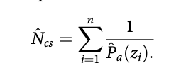
The scale parameter of the detection function becomes a function of these additional covariates (Marques & Buckland 2003). If MCDS is used, the probability of detection associated with cluster r, Pa (z,) (i = 1, 2, ..., n, where n is the total number of detected clusters) is conditional on the corresponding covariate values z,-. An estimate of cluster abundance in the covered area (corresponding to the covered strips of width 2w, i.e., extending a distance w either side of the lines) of size a is then obtained with this formula (e.g., Marques & Buckland 2003):
To estimate animal abundance, this estimate can be multiplied by an estimate of mean cluster size, using the regression method (Buckland et al. 2001: 73 - 75) to correct for size bias. We define the covered area as the area within which a systematic sample of surveyed transects was conducted, and for which we can estimate abundance using line transect sampling alone. The conventional methods for DS used in our survey rely on a set of assumptions (Buckland et al. 2001), the most important being: (1) a large number of transects are randomly allocated in the study area independently of the distribution of the population of interest; (2) all animals on the line are detected with certainty, i.e., g(0) = 1; (3) animal movement is slow with respect to observer movement; (4) distances are measured without error. An evaluation of the extent to which each of these was fulfilled is provided in the Discussion.
Analysis in programme R, package distance
The line transect data were analysed using software R (version 3.2.2, R Development Core Team 2015), partly with the Distance package (Miller 2015). Plotting and preliminary analysis of all the data with half-normal and hazard-rate detection functions showed a well-behaved detection function decreasing with distance and no evidence of any major problems. These detection functions were chosen because they provided good fit to the polar bear DS data published in Aars et al. (2009). Based on visual examinations of histograms, and in close accordance with the 2004 survey (Aars et al. 2009), we right truncated the distances beyond 1000 m to preclude fitting spurious bumps in the tail of the detection function. A number of candidate covariates were available for modelling the detection function: habitat, structure (around the position the bear was observed), cluster size and helicopter team. Their inclusion was assessed by using minimum AIC, and the overall fit was evaluated using the standard chi- square, the Kolmogorov-Smirnov and the Cramer- von Mises tests. A priori, cluster size was not expected to influence detectability, with clusters acting as single cues. Because of small sample size of families, and also because we could rarely see if a litter had one or two cubs from a distance, cluster size was scored with two categories only, lone bears or families. Both habitat and structure were believed to be potentially useful for modelling the detection function. For abundance estimation, we considered a common detection function model across strata (Pack Ice and Land), with density estimated by stratum conditional on the observed covariate values.
Correction for Pack Ice areas not covered
Fog and icing conditions during the Pack Ice survey were very challenging. Despite the allocation of three weeks to survey this area, the coverage was not even, with a non-covered gap in the western part of the study region. Further, in the east we ended up with shorter transect lines than planned running north from the ice edge, leaving much of the north-eastern part of the study region with no coverage (Fig. 1). The line transects actually flown in the Pack Ice area covered 45 009 km2, which was only 60% of the 75 562 km2 area planned to be covered. As in the 2004 survey (Aars et al. 2009), we used a ratio estimator to estimate the number of bears in the Pack Ice areas not covered by DS.
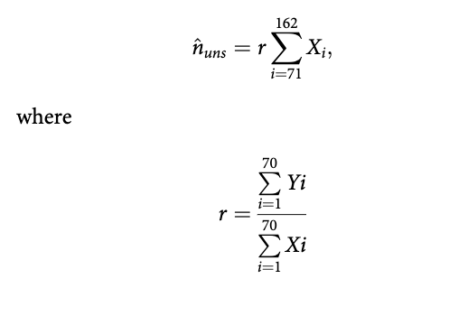
The procedure was as follows. Considering boxes encompassing line transects flown, and boxes encompassing lines or segment of lines designed for survey but not flown, we used the variable number of telemetry Argos or GPS fixes (from adult females with collars) within each box, to predict the number of bears that would have been detected had the lines been flown. Seventy transects were flown, hence we had for each of these in the covered area both the number of fixes and the number of detected bear groups. In addition, 92 boxes were encompassing both the extension of the 70 flown transects north from the point where they were terminated, and other lines not flown, with a spacing of 4.5 km between the lines. Satellite telemetry fixes have high position accuracy compared to the scale on which polar bears move. For Argos, telemetry accuracy has been estimated to be less than 1400 m for 92% of the locations for polar bears in the area collected during 1988-2000 (Mauritzen et al. 2001), and newer data based on GPS locations collected after that period are much more accurate.
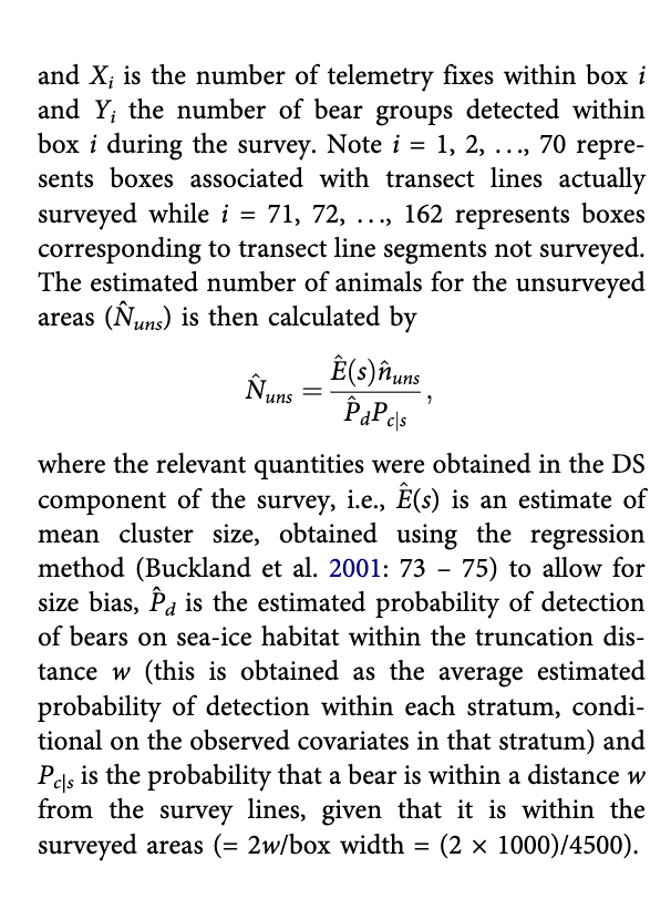
We used only positions from the period of the year when the ice edge is furthest north (July- September) from 142 different bears tracked between 1988 and 2015. Only positions north of 79°N and at least 20 km from land were considered (1570 data points). If more than one position was available for a given bear, we retained only one position for every six days to reduce dependence between bear locations (Aars et al. 2009), giving a total of 335 data points. Each point was allocated to the appropriate box, with boxes defined in terms of distance from the ice edge. In other words, a fix x km north of the ice edge in a given year would be assigned x km north of the ice edge in our survey, even if the ice edge was in a different absolute position. The number of bear groups that would have been detected if transects had been flown in the areas not surveyed, nun$, was estimated using the following ratio estimator:
Total estimate and variance estimation
The total estimated number of bears was obtained as N = Nc+Nd+Nr, where Nc is a total count (Svalbard only), Nd is the number estimated for areas covered by line transects (DS) for both Svalbard and the Pack Ice, and Nr is the number of bears in areas not surveyed in the Pack Ice area based on the ratio estimator using telemetry data. Nc, assumed to be a constant, does not contribute to the variance. To obtain estimates of variance for the estimated abundances we used a nonparametric bootstrap (9999 bootstrap resamples). Variance estimates were obtained by resampling lines within strata, as described in Buckland et al. (2001). In the case of the Pack Ice strata, the 92 line transects were resampled, along with all the information contained in them (survey data and telemetry fixes). To incorporate the variance involved in estimation for both covered and not covered areas, the bootstrap procedure had to be implemented outside Distance, using software R (version 3.2.2; R Development Core Team 2015), with Distance called from R. Therefore, for each bootstrap resample, an estimate of all random quantities involved both in the DS component and the ratio estimator component were obtained. As both detections and fixes are resampled together within the bootstrap, no assumption of independence is made between the estimate for the unsurveyed and surveyed areas when calculating the variance of the whole subpopulation. Cis were obtained by the percentile method (Buckland et al. 2001). It is theoretically superior not to bootstrap at lower levels when data are hierarchical (Davison & Hinkley 1997). Accordingly, we do not bootstrap fixes within boxes in addition to boxes.
Results
Substructure evaluated from recapture rates
We evaluated if the appropriate level for population estimation is the whole survey area including Svalbard and the Pack Ice areas north of Svalbard, or if indication of limited movement of animals between these areas supported separate estimates for each of the two areas.
Recapture rates were estimated from observation of ear tags present and identification of animals earlier marked through DNA profiles. In total, 155 biopsies were taken. Six did not have sufficient DNA to derive a genetic profile. Among the remaining 149, we found 138 different profiles, i.e., 11 individuals were biopsied twice. When excluding the duplicates, 35 of the 138 different bears had matches in the genetic database of earlier captured bears. An ear tag in at least one of the ears was seen in photographs of 26 of these 35 individuals (74.2%). Ear tags were observed on another six of the 103 individuals that had no genetic match in the database. Therefore, at least 41 of the 138 biopsied bears (29.7%) were individuals that had been marked earlier. Another 22 bears were observed where no biopsy was taken. From these bears, pictures of ears were available for 14 and not for the remaining eight. An ear tag was observed for five of the 14 (35.7%). Therefore, for the biopsied bears with a DNA profile and the bears not biopsied but with available ear pictures, a minimum of 46 of 152 (30.3%) were previously marked bears.
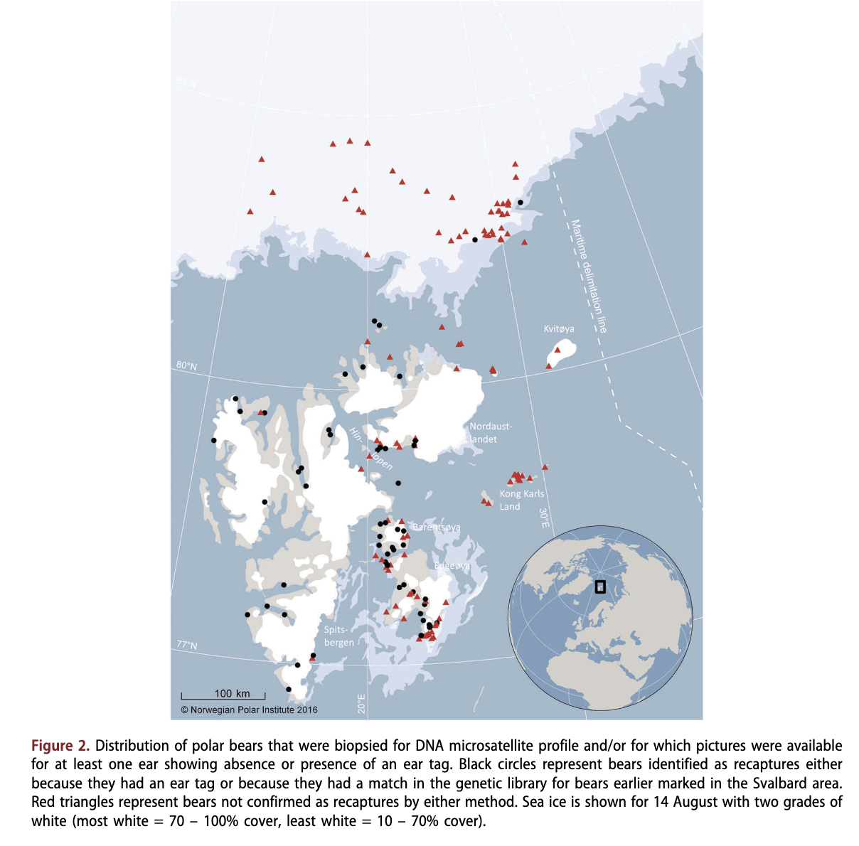
There was a striking geographic pattern in recapture probabilities (Fig. 2). In areas where capture effort has been considerable in the past 30 years, the proportion of recaptured bears varied from 88.2% (n = 17) in west Spitsbergen to 40.0% in the Hinlopen Strait north-east of Spitsbergen (n = 15), 41.7% in the northern Nordaustlandet area (n = 12) and 44.0% in the Edgeoya and Barentsoya area east of Spitsbergen (n = 50). Pooled over these areas, 51.1% (n = 94) were recaptures. None of the 20 bears biopsied at the smaller islands furthest east in Svalbard (Kong Karls Land, Kvitoya and Storoya) was a confirmed recapture. Therefore, for Svalbard, including the eastern islands, 42.1% (n = 114) of the bears were confirmed recaptures. Only two out of 44 bears (4.5%) sampled in the Pack Ice were recaptures. Below we present a separate population estimate for Svalbard and the Norwegian Pack Ice, and a total estimate for the Norwegian Arctic (Svalbard + Pack Ice). We compare these estimates with the estimates from the same areas from 2004.
Estimate
Total counts (NJ)
The number of bears counted in Svalbard in areas not covered by line transects was 68. In addition to bears we observed during our survey (n = 45, including one bear on a transect line > 1 km from the rim of a glacier), another 23 bears were: (1) in areas we considered none to be present, observed opportunistically by people in the field; (2) in the total count survey area, observed by others, and confirmed not to be seen by us; or (3) had an active satellite collar (n = 4) and were within the total count survey area but were not observed.
Line transects (NJ)
A few short lines flown on sea ice north from Nordaustlandet resulted in no observed bears. We subsequently excluded the limited sea ice in Svalbard from further analyses. Next, we evaluated the need to include glacier habitat. Data from 80 bears provided 7424 telemetry positions extracted from 114 August bear- months of which 4649 (63.0%) were on the islands. Four hundred and eighty of all positions (6.4%) were on glaciers. Only 67 of these positions (0.9% of all positions and 1.4% of the positions on islands) were farther in than 1 km from the rim of the glaciers. Based on that knowledge, we defined habitat Land as bare land and glaciers < 1 km from the rim, and excluded
observation of bears on the remaining parts of all glaciers from the line transect estimates. This means that we might underestimate the subpopulation size by less than 1% by excluding the inner parts of the glaciers. This seems reasonable given the required effort that would otherwise be necessary to estimate such a small fraction of the overall subpopulation. We flew about 10 950 km in 279 transect lines divided between the Pack Ice (about 7700 km) and Land (about 3250 km), see Table 1. The coverage was close to the study design for Land (Fig. 1). For the Pack Ice, large areas that were planned to be surveyed were not covered due to long periods of fog and icing conditions. These areas were
Table 1. Estimates of polar bear density and abundance for strata Pack Ice and Land (islands including a belt of glaciers 1 km in from their rim) in the areas covered by line transect DS. Estimates are based on the model with the lowest AIC (Hazard Rate key function) and Strata (Pack Ice or Land) as covariate.
Strata | km lines | Obsa | Db | D 95% Cl | N' | N 95% Cl | km2 |
Land | 3254 | 88 | 1.9 | (1.3; 2.9) | 196 | (131; 295) | 10 124 |
Pack Ice | 7733 | 37 | 1.1 | (0.6; 1.9) | 478 | (264; 866) | 45 009 |
Total | 10 987 | 125 | 1.2 | (0.7; 2.1) | 674 | (432; 1053) | 55 133 |
aNumber of distance observations used to fit the curves but including the 5% truncated observations. bBear density (per 100 km2). 'Predicted number of bears in covered areas.
mostly found furthest east in the Pack Ice area, where most transects were short and mostly covered the areas close to the ice edge (Fig. I).
A total of 125 bear groups were observed on line transects. Of these, 100 were lone bears. The remaining 25 were family groups consisting of a female with either one (n = 14) or two cubs (n = 11). The maximum perpendicular distance was 2696 m (Fig. 3). After truncation (at 1000 m), 32 (out of 37) observations and 70 (out of 88) were kept for further analyses for the Pack Ice and Land strata, respectively. After truncation, the average group size was 1.438 (SE 0.133) for the former and 1.243 (SE 0.075) for the latter.
Based on the model selection process, we ended up with a simple Hazard Rate model with strata (Land, Pack Ice) as the only covariate (Table 2, Fig. 3). Neither cluster size (lone bears or families) nor habitat structure improved the fit (see Table 2). As anticipated, bears on Land had a higher probability of detection (P = 0.69) than bears in the Pack Ice (P = 0.28), Fig. 3. The estimated number of bears within the covered areas in the Pack Ice area was 478 (95% CI = 264 - 866). The estimate for Land was 196 (95% CI = 131 - 295). The total estimate for the areas covered by DS was therefore 674 (95% CI = 432 - 1053).
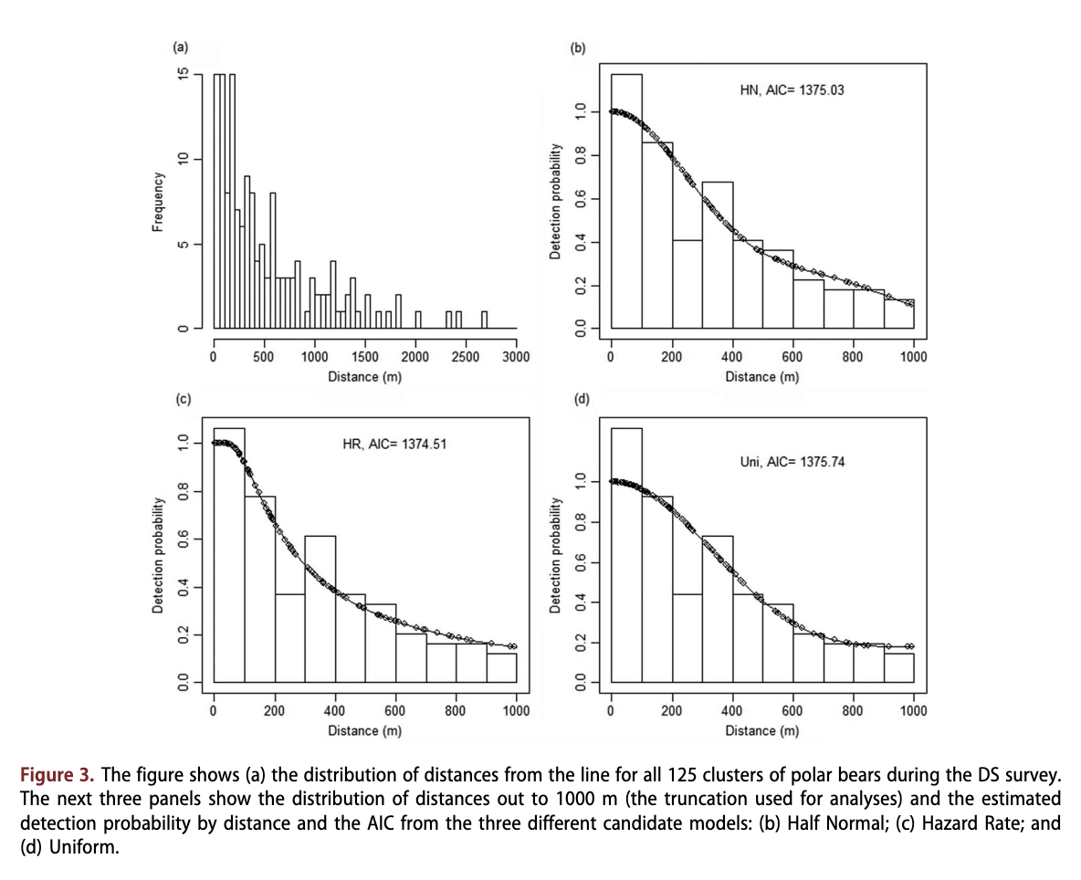
Table 2. Details for DS models including different covariates. Shown are AIC values for 10 different models with key function (Key F) being either hazard rate (HR) or half normal (HN), and different combinations of covariates. The covariates considered in the models were: habitat (Strata, either Land or Pack Ice), family (Fam, either adult female with cub(s) or lone bear) and structure (Str, factor with three levels). Models are sorted with increasing AIC, and change in AIC (dAIC) reported relative to the model with lowest AIC. Goodness of fit measures are presented with a Kolmogorov-Smirnov (Pks) and a Cramer-von Mises test (PCvM).
Key F | Strata | Fam | Str | AIC | dAIC | Pks | PCvM |
HR | X |
|
| 1365.07 | 0.00 | 0.989 | 0.979 |
HN | X |
|
| 1366.02 | 0.95 | 0.729 | 0.629 |
HN | X | X |
| 1366.44 | 1.37 | 0.739 | 0.596 |
HR | X | X |
| 1366.69 | 1.62 | 0.948 | 0.956 |
HN | X |
| X | 1367.67 | 2.60 | 0.846 | 0.711 |
HR | X |
| X | 1367.82 | 2.75 | 0.985 | 0.964 |
HR |
|
|
| 1374.51 | 9.44 | 0.994 | 0.994 |
HN |
|
|
| 1375.03 | 9.96 | 0.850 | 0.952 |
HN |
|
| X | 1377.58 | 12.51 | 0.283 | 0.270 |
HR |
|
| X | 1378.33 | 13.26 | 0.998 | 0.991 |
Number of bears in the Pack Ice areas not covered In the Pack Ice, the 70 transect lines that were flown had 32 detected groups within the truncation distance, and the 70 boxes associated with these 70 transects had 206 GPS fixes from collared bears. The ratio estimator (32/206) was thus 0.155. The area we failed to cover (not including the small areas that we found natural to include in the DS area for density estimation, Fig. 1) had 129 GPS fixes, and from the ratio estimator, an estimated 20 groups would have been detected had the area been covered (129 * 0.155). From this, 231 bears were estimated to be in the Pack Ice uncovered areas.
Estimated number of bears
The total estimate N = Nc+Nd+Nr was 68 + 674 + 231 = 973 (Table 3) with a bootstrap (9999 runs) 95% CI of 665 - 1884. The separate estimate for Svalbard was 68 (Nc) +196 (95% CI = 131 - 295) = 264 (95% CI = 199 - 363). The estimated number of bears for the Norwegian Pack Ice (478 in the DS covered area + 231 in the not covered area) was 709. The 95% CI was 334 - 1026. Although considerably higher than the 444 estimated for the Norwegian Pack Ice in 2004, uncertainty in that estimate was also considerable (95% CI = 282 - 606, see Table 3), i.e., the two Cis had a considerable overlap. The estimates from 2004 for Norwegian/Svalbard Land (Land + Glacier according to the subdivision in Aars et al. 2009) provided a very similar and low figure (n = 241) for these supposed mainly local bears, with a 95% CI of 153 - 329 (Table 3). All of the Cis for changes in N between 2004 and 2015 included zero (Table 3).
Table 3. Estimates of polar bear abundance in 2015 for the Norwegian part of the Barents Sea for Svalbard, for the Pack Ice and the total. For comparison, results for the 2004 survey (Aars et al. 2009) are also provided. Cis for the same subcomponents for the 2004 survey were not directly available. We calculated these here based on summing the variance for estimates of (a) distance sampled Pack Ice area and (b) area not covered in the Pack Ice, estimated based on telemetry positions, and summing the variance for (c) glacier in Svalbard and (d) land area in Svalbard for the Land. See Aars et al. (2009) for details. A Gaussian distribution was assumed both for the estimates of the 2004 Cis and for the Cl of the change in the N between surveys.
| 2004 | 2015 | Change, 2004 to 2015 | |||
N | N 95% Cl | N | N 95% Cl | Д N | Д N 95% Cl | |
Svalbard | 241 | (153, 329) | 264 | (199, 363) | 23 | (-97, 143) |
Pack Ice | 444 | (282, 606) | 709 | (334, 1026) | 265 | (-117, 647) |
Total | 685 | (501, 869) | 973 | (665, 1884) | 288 | (-349, 925) |
Demographic population structure
Using observational and genetic data from bears from both DS areas and total count areas, we can calculate relevant demographic quantities. Among 133 independent bears observed in the field for which assumed sex was recorded, and for which we also had a genetic profile, 10 were scored wrongly in the field if we assume the genetic result was correct. This gives a 92.5% correct field sex score. From genetics, 142 different individuals were identified as 62 females and 80 males. Another assumed 14 females and seven males were added based on field scores and pictures. Only three independent bears were not scored to sex by any method. This gives an estimated female sex ratio of 0.466 (95% CI = 0.388 - 0.546). Twenty-one females were with one (n = 14) or two (n = 7) cubs of the year. Another 11 were with one (n = 6) or two (n = 5) yearlings. The 28 cubs of the year and the 16 yearlings constitute 13.3% and 7.6%, respectively, of the total 210 different individuals recorded, and therefore 44 (21.0%) dependent cubs. The 21 and 11 adult females with cubs of the year and yearlings constituted, based on the female proportion of 0.466 among independent observed bears, 27.1% and 14.2%, respectively, of the subadult and adult females. Thus, 41.3% of the females were with dependent cubs. The rates were similar for Svalbard and the Pack Ice.
Discussion
Recognizing the correct geographical units for estimates
The recapture rates based on individuals identified from DNA analyses of biopsy tissue samples and the presence of ear tags on photographed bears observed during the surveys demonstrated that bears in Svalbard are separated to a large degree from bears found further north in the Pack Ice in the autumn. The results of the present study demonstrate that most bears living in Svalbard in autumn are local bears also inhabiting the area in spring (given that original captures in earlier years with only a few exceptions were conducted in Svalbard in late March or April). This is in accordance with data from satellite tagged females as well as morphometric data from skulls which have disclosed a substructure in the Barents Sea subpopulation (Mauritzen et al. 2001; Pertoldi et al. 2012). We have also shown that very few of the bears in the Pack Ice are among those likely to be captured in Svalbard in spring. We conclude that in years when the Pack Ice is located in areas separated from the Svalbard islands, a local Svalbard stock of polar bears will be a natural ecological unit with some degree of isolation from other parts of the Barents Sea subpopulation. Therefore, estimates of size, trend and other demographic rates may best be assessed for this ecotype separately. The bears in the Pack Ice should be assessed as a part of a Russian-Norwegian pelagic Barents Sea ecotype. The reproductive barrier between the two ecotypes has until recently been low (Zeyl et al. 2010). However, pelagic bears visiting Svalbard typically den in the eastern parts of the archipelago, and in years with late sea-ice freeze-up in these areas, none or few females reach the islands for winter maternity denning (Derocher et al. 2011; Aars 2013). It is likely that the two ecotypes currently experience a fast decrease in overlap both in area and time. We anticipate that in the future, the majority of the pelagic bears will den in Franz Josef Land as they fail to reach the traditional and very important denning areas in eastern Svalbard (Andersen et al. 2012). A dramatic shift in available preferred polar bear sea-ice habitat many degrees northward from Svalbard for longer periods of the year through the last decades has been documented (Lone et al. 2017).
Survey estimates
The estimated numbers of polar bears in Svalbard in August 2004 and 2015 were similar. Together with the recapture rates, these estimates demonstrate that most of these bears are likely local bears staying in the area year round and indicate that the Svalbard ecotype only represents a minor part of the Barents Sea subpopulation that was estimated to be approximately 2650 bears in 2004 (Aars et al. 2009). The number of bears in Svalbard in autumn will likely vary considerably between years, depending on the location of the sea-ice edge. In years with more sea ice around Svalbard, a higher number of bears will be found here as a larger proportion of the pelagic bears will be in the area. Several of the bears encountered during the survey in the eastern islands of Svalbard in 2015 were likely pelagic bears that had failed to follow the retreating sea-ice edge in summer. We collared three females on Kongsoya and Kvitoya (Fig. 1) in the eastern part of Svalbard with GPS satellite transmitters during the survey. Two of these swam from Kongsoya and west to Nordaustlandet 80 km away, using just above 30 hours. The third swam from Kvitoya (Fig. 1), first 58 km west to a smaller island, then another 84 km to the Pack Ice, reached after four and a half days. One female was also sighted first on Kongsoya in early August and then in the Pack Ice 310 km away in late August (identified from a biopsy DNA profile). We conclude that most of the bears that were in Svalbard in August in 2015 belonged to the local ecotype and that the pelagic ecotype mostly occupied the Pack Ice area. It is not possible to quantify the proportion of the pelagic polar bears that were in Svalbard during the survey in 2015. The combined data on recapture rates and from what we know about collared females indicate that in years when the Pack Ice is located far north of Svalbard, as was the case in both 2004 and 2015, the pelagic bears are, if not in the Pack Ice area, mainly encountered on the very eastern parts of Svalbard. The number of bears confined to Svalbard seems not to have changed significantly over the last decade, despite experiencing a period with historically little sea ice—a reduction of about five months of the sea-ice season from the late 1970s (Stern & Laidre 2016). This indicates that the local Svalbard bears survive and reproduce under conditions with much less habitat available than was the case historically and until quite recently. The population may not yet have reached the current carrying capacity despite having been protected for more than 40 years. Aars et al. (2009) pointed out that the subpopulation historically may have been much larger to sustain a very high annual take of bears over 100 years up to the protection in 1973.
The estimate of about 700 bears in the Norwegian Pack Ice in 2015 was larger than in 2004 but the change was not significant. The bears in the Pack Ice area have no natural barrier to the east or to the west, but movement during August is assumed to be limited and not expected to be directional (Mauritzen et al. 2003). However, the density along the ice edge was observed to vary a lot in both 2004 and 2015. In 2004 many more bears were found in the Russian Pack ice area than in the Norwegian part. In 2015, most bears in the Pack Ice were seen in the eastern areas not far from the Russian border. Caution must therefore be taken when discussing trends for this ecotype.
Bear densities
The distribution of bears on land in Svalbard is clumped, with 1.9 per 100 km2 in the DS covered areas, but on average the estimate in 2015 only equals 0.43 bears per 100 km2 for all land areas. This is about twice as high as in Foxe Basin, Canada, during the sea-ice-free summer (Stapleton et al. 2016) and in the southern Hudson Bay (Obbard et al. 2015). The density we found in the Pack Ice areas covered by DS, of 1.1 bears per 100 km2, is also relatively high compared to, e.g., Arctic Canada in April (average 0.41 bears per 100 km2; Taylor & Lee 1995) and to the Chukchi Sea in August 2000 (average 0.68 bears per 100 km2; Evans et al. 2003). Our results from 2015, combined with the results from the 2004 survey (Aars et al. 2009), indicate that polar bear densities in the Barents Sea area are relatively high. This is interesting taking into account our belief that the historical population size must have been considerably higher than today in order to provide a catch of an average > 300 bears annually over 100 years (Lons 1970; for discussion see Aars et al. 2009). Spatial variability in distribution of collared female polar bears in the Pack Ice is under study (Lone et al. 2017). The distribution can to a large degree be explained by a sea-ice-specific resource selection function model.
Demography
The use of DNA markers allowed us to sex bears and also to show that we identified more than 90% of subadults and adults to the correct sex from visual observation. A close to 1:1 sex ratio (estimated 46.7% females) in a population that is not hunted indicates that natural survival of adult males and females may be similar. A sudden non-linear drop in survival of adult male polar bears with increasing periods of food stress due to habitat loss has been proposed based on population models (Molnar et al. 2010). Given that we sampled more males than females, our data do not provide evidence that such a critical point has been reached in the Barents Sea area yet. Identification of sex allowed us to estimate the fraction of females that were with cubs (41%). As females in this area usually do not have cubs before the age of six (Derocher 2005), and the estimate includes subadults (two- to five-year-olds), the proportion of mature females that were with cubs is higher, and not possible to estimate. The proportion of cubs and yearlings in the population of 21% is somewhat lower than 28% recorded in the survey in 2004 (Aars et al. 2009), but well within the range of typical values for viable polar bear populations. Cubs and yearlings represented 25% of bears observed in Foxe Basin (Stapleton et al. 2016) and 28% in southern Hudson Bay (Obbard et al. 2015) during aerial surveys in autumn. In contrast, in western Hudson Bay, an area where loss of sea-ice habitat has been demonstrated to have profound effects on demographic rates (e.g., Regehr et al. 2007; Lunn et al. 2016), only 10% of the observed bears in a comparable aerial survey were dependent cubs (Stapleton et al. 2014). Derocher (2005) found that adult females in Svalbard produced less cubs in years following years with milder weather. Annual capturerecapture data from Svalbard indicate a negative time trend in reproduction, with a predicted reduction from above 0.75 to less than 0.5 cubs per adult female in April over the last 20 years, but that annual variation is large (MOSJ 2017). The considerable interannual variation in production and cub survival has implications for assessment of population size estimates. In 2004, the average bear cluster size was 1.39, compared to 1.44 for the Pack Ice DS data, and 1.24 for Svalbard DS data in 2015. Hence, there is no evidence that the fraction of cubs in these two years might have been very different or have influenced the trend analyses.
Assumptions and possible sources of bias
In Svalbard, some bears would necessarily have been in areas covered neither by line transects nor total counts. However, telemetry data combined with information on where people observed polar bears during the survey suggest that few bears were distributed in areas of glaciers and land that were not covered by surveys. More bears may have been swimming in the ocean. Data from female adults that have had data loggers show that they spent about 4% of the time in water in August (Norwegian Polar Institute, unpubl. data). Swimming bears would in most cases be outside the survey area and not available for counting and would contribute to a negatively biased estimate. We think that the total count of 68 bears in Svalbard accounts for most of the bears in the covered area. Bears are in general easily detectable in most terrain when there is no snow, and it was not snowing during the survey.
For the areas covered by line transects, detection of bears was considerably higher for Land (in Svalbard) than for the Pack Ice. Because of the limited number of observations we did not find a good way to evaluate g(0), the proportion of bears detected “on” the line. The survey method in 2015 was, however, consistent with the 2004 survey, making it likely that an underestimate due to g(0) < 1 would not be very different between the two surveys. We concluded (Aars et al. 2009) that g(0) likely was very close to 1 on land, close to 1 in areas with flat sea ice (most of the Pack Ice, except some areas close to the ice edge), and that the areas with very screwed sea ice where g (0) could have been considerably lower than 1 only constituted a very minor part of the total survey area. g(0) has been estimated by double observer platforms in other line transect DS surveys of polar bears. While Stapleton et al. (2016) estimated g(0) to be close to 1, Obbard et al. (2015) estimated it to be close to 0.8. Both studies were performed in areas where bare land provided a background in general considerably darker than the bears. The failure to evaluate g(0) in our study introduces a bias we cannot quantify. The bias is more likely to be higher in the Pack Ice where the colour of bears and of the background is more similar than on land. We assume the bias is not very different during the 2015 survey from what it was during the 2004 survey. Five of the 12 observers (including pilots) were the same during these surveys, helicopters were of the same model and the methods were consistent. We therefore assume that the two surveys are directly comparable.
Movement of bears could induce biases in several ways. If movement is directional on a larger geographical scale, it could lead to a bias if the survey covers different areas in different periods while the movement of the bears leads to changing densities in these areas. In western Svalbard, we believe bears mostly stayed within the same area for the whole survey period. On the islands farthest to the east we do know that several bears swam from the islands to Nordaustlandet or to the Pack Ice (see above). We do find it likely that pelagic bears in the area leave the islands in the weeks after the sea ice disappears, to reach the Pack Ice to the north with better hunting habitat. Those bears will be outside the survey area when swimming and bias the estimate down. However, with two teams, Svalbard was surveyed during the first three weeks of August, while the Pack Ice was surveyed some days in early August and some days at the end of August. Also, the total number of pelagic bears in eastern Svalbard was assumed to be very modest compared to the estimated number in the Pack Ice. Movement would also bias estimates (down) if the distance from the line to the bears increased because bears fled away from the helicopter before they were spotted (or they were not seen, because they were further away). Given the high speed of the helicopter (185 km/h) relative to the bear, and more important, the fact that we only rarely spotted bears running or looking like they were reacting to the helicopter when first seen, we assume this is not a problem. Bears do react when they are just below the helicopter (“on the line”), but then they may move in any direction relative to the line, and also they are often seen at the moment they start reacting. Out of 11 bears we observed twice during the survey on Svalbard (confirmed by DNA profiles), three were observed twice from different survey lines within an hour. Two of these were within the truncation distance at both sightings. With 3 km between lines, and truncation 1 km to each side, bears would be able to reach the next survey line from time to time, depending on the length of each survey line (how long it takes for the helicopter to reach the next line at a point close to the original observation of any bear moving from a line). In general, we did not have the impression that bears moved away from the line as a response to the helicopter. We consider this source of bias as minor. If measurement of the distance from the line to the bear at the point it was when first seen was inaccurate and biased, this would also bias any estimate. The method used (flying out to the position taking a GPS position) was evaluated through a study by Marques et al. (2006) and shown to be very accurate.
A bias could also be caused by different coverage of different terrain types with different densities of bears, if not known and accounted for. Lines were laid to sample terrain types as evenly as possible on islands with changing topography. A dense and large number of lines in the areas covered makes it unlikely that this is an issue.
The area with the largest potential for a bias is the Pack Ice where the density estimate was based on the ratio estimator from collared adult female bears from several different years. The main assumption behind this method is that bears of both sexes and all ages are represented by the adult collared females. A few studies have looked at how polar bear males move compared to females. Laidre et al. (2013) found that in east Greenland movement pattern was sex specific on a smaller scale, but habitat preference did not differ.
Conclusion
Nowhere in the range of polar bears has a faster loss of sea ice from climate change been recorded than in the Barents Sea area. With a continuing fast loss of sea ice expected, it is a question of time before a declining carrying capacity will equal that of a subpopulation in recovery from the overharvest before protection in 1973. The most significant knowledge from this study is that Svalbard seems to host a local ecotype of the Barents Sea subpopulation of polar bears which constitute only a few hundred individuals. These bears experience different challenges than the much higher number of bears living in the Pack Ice area. Future monitoring and management of the Barents Sea subpopulation should therefore take this substructure into account. Current knowledge of the ecology of this subpopulation, which is based on Norwegian studies, applies mostly to the Svalbard bears. A change in the monitoring programme is needed to provide better management-relevant knowledge for the pelagic Barents Sea bears. The level of substructure between the two ecotypes is likely to increase in the coming years.
Acknowledgements
Vidar Bakken, Rupert Krapp and Jade Garcia contributed to field planning and during the survey. Morten Ekker, Oystein Overrein and Dag Vongraven were involved in the initial work to actualize the survey and pre-survey discussions. Airlift AS contributed as always with top experienced teams of pilots (Anders Bjorgum, Arvid Holen and Ola Rugland) and mechanics (Dante Fontana and Gunnar Nordahl). Thanks also to the crews of the RV Lance and KV Svalbard, and to all marine mammal observers on the ships for fruitful discussions during the surveys. The governor of Svalbard provided the necessary permits for operation in Svalbard. The Norwegian Animal Research authorities in Norway permitted handling of polar bears including biopsy darting.
Disclosure statement
No potential conflict of interest was reported by the authors.
Funding
This study was funded by the Norwegian Ministry of Climate and the Environment. TAM is grateful for partial support by Centro de Estatistica e Aplicatjoes da Universidade de Lisboa, funded by the Fundatjao para a Ciencia e a Tecnologia, Portugal, through the project UID/ MAT/00006/2013.
References
- Aars J. 2013. Variation in detection probability of polar bear maternity dens. Polar Biology 36, 1089-1096.
- Aars J., Marques T.A., Buckland S.T., Andersen M., Belikov S., Boltunov A. & Wiig 0. 2009. Estimating the Barents Sea polar bear subpopulation size. Marine Mammal Science 25, 35-52.
- Amstrup S.C. 2003. Polar bear, Ursus maritimus. In G.A. Feldhamer et al. (eds.): Wild mammals of North America: biology, management, and conservation. Pp. 587-610. Baltimore: Johns Hopkins University Press.
- Andersen M., Derocher A.E., Wiig 0. & Aars J. 2012. Polar bear (Ursus maritimus) maternity den distribution in Svalbard, Norway. Polar Biology 35, 499-508.
- Bidon T., Frosch C., Eiken H., Kutschera V., Hagen S., Aames S., Fain S., Janke A. & Hailer F. 2013. A sensitive and specific multiplex PCR approach for sex identification of ursine and tremarctine bears suitable for non-invasive samples. Molecular Ecology Resources 13, 362-368.
- Buckland S.T., Anderson D.R., Bumham K.P., Laake J.L., Borchers D.L. & Thomas L. 2001. Introduction to distance sampling. Oxford: Oxford University Press.
- Buckland S.T., Rexstad E., Marques T. & Oedekoven C. 2015. Distance sampling: methods and applications. Cham, Switzerland: Springer International Publishing Switzerland.
- Davison A.C. & Hinldey D.V. 1997. Bootstrap methods and their application. Cambridge: Cambridge University Press.
- Derocher A.E. 2005. Population ecology of polar bears at Svalbard, Norway. Population Ecology 47, 267-275.
- Derocher A.E., Andersen M., Wiig 0., Aars J., Hansen E. & Biuw M. 2011. Sea ice and polar bear den ecology at Hopen Island, Svalbard. Marine Ecology-Progress Series 441, 273-279.
- Durner G.M., Douglas D.C., Nielson R.M., Amstrup S.C., McDonald T.L., Stirling L, Mauritzen M., Bom E.W., Wiig 0., De Weaver E., Serreze M.C., Belikov S.E., Holland M.M., Maslanik J., Aars J., Bailey D.A. & Derocher A.E. 2009. Predicting 21st-century polar bear habitat distribution from global climate models. Ecological Monographs 79, 25-58.
- Ekker M., Aars J., Haugan M., Jernquist E., Stokke E., Vongraven D. & Wiig 0. 2013. Norsk handlingsplan for isbjorn. (Norwegian action plan for polar bears.) Trondheim: Norwegian Environmental Agency.
- Evans T.J., Fischbach A., Schliebe S., Manly B., Kalxdorff S. & York G. 2003. Polar bear aerial survey in the Eastern Chukchi Sea: a pilot study. Arctic 56, 359-366.
- Laidre K.L., Bom E.W., Gurarie E., Wiig 0., Dietz R. & Stern H. 2013. Females roam while males patrol: divergence in breeding season movements of pack-ice polar bears (Ursus maritimus). Proceedings of the Royal Society B-Biological Sciences 280, article no. 20122371, doi: 10.1098/rspb.2012.2371.
- Laidre K.L., Stern H., Kovacs K.M., Lowry L., Moore S.E., Regehr E.V., Ferguson S.H., Wiig 0., Boveng P., Angliss A.P., Born E.W., Litovka D., Quakenbush L., Lydersen C., Vongraven D. & Ugarte F. 2015. A circumpolar assessment of Arctic marine mammals and sea ice loss, with conservation recommendations for the 21st century. Conservation Biology 29, 724-737.
- Laidre K.L., Stirling I., Lowry L.F., Wiig 0., Heide- Jorgensen M.P. & Ferguson S.H. 2008. Quantifying the sensitivity of Arctic marine mammals to climate-induced habitat change. Ecological Applications 18, S97-S125.
- Larsen T.S. 1986. Population biology of the polar bear (Ursus maritimus) in the Svalbard area.. Norsk Polarinstitutt Skrifter 184. Oslo: Norwegian Polar Institute.
- Lone K., Merkel B., Lydersen C., Kovacs K.M. & Aars J. 2017. Sea ice resource selection models for polar bears in the Barents Sea subpopulation. Ecography 40, Early View, doi: 10.1111/ecog.03020.
- Lono O. 1970. The polar bear (Ursus maritimus Phipps) in the Svalbard area. Norsk Polarinstitutt Skrifter 149. Oslo: Norwegian Polar Institute.
- Lunn NJ., Servanty S., Regehr E.V., Converse SJ., Richardson E. & Stirling I. 2016. Demography of an apex predator at the edge of its range: impacts of changing sea ice on polar bears in Hudson Bay. Ecological Applications 26, 1302-1320.
- Marques F.F.C. & Bucldand S.T. 2003. Incorporating covariates into standard line transect analyses. Biometrics 59, 924-935.
- Marques T.A., Andersen M., Christensen-Dalsgaard S.N., Belikov S., Boltunov A., Wiig 0., Buckland S.T. & Aars J.
2006. Comparing distance estimation methods in a helicopter line transect survey. Wildlife Society Bulletin 34, 759-763. - Mauritzen M., Derocher A.E., Pavlova O. & Wiig 0. 2003. Female polar bears, Ursus maritimus, on the Barents Sea drift ice: walking the treadmill. Animal Behaviour 66, 107- 113.
- Mauritzen M., Derocher A.E. & Wiig 0. 2001. Space-use strategies of female polar bears in a dynamic sea ice habitat. Canadian Journal of Zoology - Revue Canadienne De Zoologie 79, 1704-1713.
- Miller D.L. 2015. Distance: distance sampling detection function and abundance estimation. R package version 0.9.3. Accessible on the internet at https://CRAN.R-project.org/package=Distance
- Molnar P.K., Derocher A.E., Thiemann G.W. & Lewis M.A. 2010. Predicting survival, reproduction and abundance of polar bears under climate change. Biological Conservation 143, 1612-1622.
- MOSJ (Environmenal Monitoring of Svalbard and Jan Mayen) 2017. Polar bear (Ursus maritimus). Recruitment graphs accessed on the internet at http://www.mosj.no/en/fauna/marine/polar-bear.html on 19 July 2017.
- Obbard M.E., Stapleton S., Middel K.R., Thibault I., Brodeur V. & Jutras C. 2015. Estimating the abundance of the Southern Hudson Bay polar bear subpopulation with aerial surveys. Polar Biology 38, 1713-1725.
- Obbard ME., Thiemann G.W., Peacock E. & DeBiuyn T.D. (eds.) 2010. Polar bears. Proceedings of the 15th working meeting of the IUCN Polar Bear Specialist Group, 29 June-3 July 2009. Copenhagen, Denmark. Occasional Paper of the IUCN Species Survival Commission 43. Gland: International Union for Conservation of Nature and Natural Resources.
- Olsen G.H., Mauritzen M., Derocher A.E., Sormo E.G., Skaare J.U., Wiig 0. & Jenssen B.M. 2003. Space-use strategy is an important determinant of PCB concentrations in female polar bears in the Barents Sea. Environmental Science & Technology 37, 4919-4924.
- Pagano A.M., Peacock E. & McKinney M.A. 2014. Remote biopsy darting and marking of polar bears. Marine Mammal Science 30, 169-183.
- Pertoldi C., Sonne C., Wiig 0., Baagoe HJ., Loeschcke V. & Bechshoft T.0. 2012. East Greenland and Barents Sea polar bears (Ursus maritimus): adaptive variation between two populations using skull morphometries as an indicator of environmental and genetic differences. Hereditas 149, 99-107.
- Prestrud P.S. & Stirling I. 1994. The international polar bear agreement and the current status of polar bear conservation. Aquatic Mammals 20, 113-124.
- R Development Core Team. 2015. R: a language and environment for statistical computing. Vienna: R Foundation for Statistical Computing.
- Regehr E.V., Hunter C.M., Caswell H., Amstrup S.C. & Stirling I. 2010. Survival and breeding of polar bears in the southern Beaufort Sea in relation to sea ice. Journal of Animal Ecology 79, 117-127.
- Regehr E.V., Laidre K.L., Ak^akaya H.R., Amstrup S.C., Atwood T.C., Lunn NJ., Obbard M., Stern H., Thiemann G.W. & Wiig 0. 2016. Conservation status of polar bears (Ursus maritimus) in relation to projected sea-ice declines. Biology Letters 12, article no. 20160556, doi: 10.1098/rsbl.2016.0556.
- Regehr E.V., Lunn NJ., Amstrup S.C. & Stirling I. 2007. Effects of earlier sea ice breakup on survival and population size of polar bears in western Hudson Bay. Journal of Wildlife Management 71, 2673-2683.
- Stapleton S., Atkinson S., Hedman D. & Garshelis D. 2014. Revisiting western Hudson Bay: using aerial surveys to update polar bear abundance in a sentinel population. Biological Conservation 170, 38-47.
- Stapleton S., Peacock E. & Garshelis D. 2016. Aerial surveys suggest long-term stability in the seasonally ice-free Foxe Basin (Nunavut) polar bear population. Marine Mammal Science 32, 181-201.
- Stern H. & Laidre K.L. 2016. Sea-ice indicators of polar bear habitat. The Cryosphere 10, 1-15.
- Stirling I. & Derocher A. 2012. Effects of climate warming on polar bears: a review of the evidence. Global Change Biology 18, 2694-2706.
- Taylor M. & Lee J. 1995. Distribution and abundance of Canadian polar bear populations - a management perspective. Arctic 48, 147-154.
- Thomas L., Buckland S.T., Rexstad E., Laake J.L., Strindberg S., Hedley S.L., Bishop J.R.B., Marques F. F.C.&. & Burnham K.P. 2006. Distance software: design and analysis of distance sampling surveys for estimating population size. Journal of Applied Ecology 47, 5-14.
- Van Beest F., Aars J., Routti H., Lie E., Andersen M., Pavlova V., Sonne C., Nabe-Nielsen J. & Dietz R. 2016. Spatiotemporal variation in home range size of female polar bears and correlations with individual contaminant load. Polar Biology 39, 1479-1489.
- Wiig 0., Amstrup S., Atwood T., Laidre K., Lunn N.. Obbard M., Regehr E. & Thiemann G. 2015. Ursus maritimus. The IUCN Red List of threatened species 2015, e.T22823A14871490, doi: 10.2305/IUCN.UK. 2015-4.RLTS.T22823A1487149O.en. Accessed on the internet at http://www.iucnredlist.Org/details/22823/0 on 27 May 2016
- Wiig 0. & Derocher A. 1999. Application of aerial survey methods to polar bears in the Barents Sea. In G.G.W. Gamer et al. (eds.): Marine mammal survey and assessment methods. Proceedings of the symposium on surveys, status and trends of marine mammal populations/Seattle/ Washington/USA/25-27 February 1998. Pp. 27-36. Rotterdam: A.A. Balkema.
- Zeyl E., Aars J., Andersen M., Ehrich D., Bachmann L. & Wiig 0. 2010. Different space-use strategies do not lead to genetic subdivision of the Barents Sea polar bear population. In E. Zeyl: Population genetics of polar bears (Ursus maritimus) in the Svalbard area. PhD thesis, Faculty of Mathematics and Natural Sciences, University of Oslo.
- Zeyl E., Aars J., Ehrich D. & Wiig 0. 2009. Families in space: relatedness in the Barents Sea population of polar bears (Ursus maritimus). Molecular Ecology 18, 73
Related Articles
C. Leah Devlin
Martyn E. Obbard
Christopher Di Corrado
João Franco
Roger Pimenta
et al.
Karen Lone
Jon Aars
Christian Lydersen
Kit M. Kovacs
et al.
Christian Lydersen
Kit M. Kovacs
Jade Vaquie-Garcia
Espen Lydersen
et al.
Herdis M. Gjelten
Øyvind Nordli
Ketil Isaksen
Eirik J. Førland
et al.