This article is published under a Creative Commons license and not by the author of the article. So if you find any inaccuracies, you can correct them by updating the article.

Characterization of sea-ice kinematic in the Arctic outflow region using buoy data


Ruibo Lei
Petra Heil
Jia Wang
Zhanhai Zhang
Qun Li
Na Li
Published: Jan. 27, 2016
Latest article update: Aug. 13, 2023
This article is published under the license


Abstract
Data from four ice-tethered buoys deployed in 2010 were used to investigate sea-ice motion and deformation from the Central Arctic to Fram Strait. Seasonal and long-term changes in ice kinematics of the Arctic outflow region were further quantified using 42 ice-tethered buoys deployed between 1979 and 2011. Our results confirmed that the dynamic setting of the transpolar drift stream (TDS) and Fram Strait shaped the motion of the sea ice. Ice drift was closely aligned with surface winds, except during quiescent conditions, or during short-term reversal of the wind direction opposing the TDS. Meridional ice velocity south of 85°N showed a distinct seasonal cycle, peaking between late autumn and early spring in agreement with the seasonality of surface winds. Inertia-induced ice motion was strengthened as ice concentration decreased in summer. As ice drifted southward into the Fram Strait, the meridional ice speed increased dramatically, while associated zonal ice convergence dominated the ice-field deformation. The Arctic atmospheric Dipole Anomaly (DA) influenced ice drift by accelerating the meridional ice velocity. Ice trajectories exhibited less meandering during the positive phase of DA and vice versa. From 2005 onwards, the buoy data exhibit high Arctic sea-ice outflow rates, closely related to persistent positive DA anomaly. However, the long-term data from 1979 to 2011 do not show any statistically significant trend for sea-ice outflow, but exhibit high year-to-year variability, associated with the change in the polarity of DA.
Keywords
Fram Strait, sea ice, Arctic Ocean, transpolar drift stream, dipole anomaly, kinematics
Hilmer & Jung (2000) found that the correlation between the NAO and sea-ice export through the Fram Strait changed from zero correlation (1958–1977) to about 0.7 (1978–1997). NAO characterizes the sea-level pressure (SLP) difference between the Icelandic Low and the Azores High and can modulate the zonal wind there. It does not directly identify the strength of the Arctic atmospheric circulation. Analysing data from 1989 to 2009, Vihma et al. (2012) found that compared with the AO and the DA, the NAO accounts for less of the interannual variability of sea-ice drift in the outflow region of Arctic Ocean. The AO can modulate the orientation of TDS, and consequently the sea-ice export into Fram Strait (Vihma et al. 2012; Kwok et al. 2013). Rigor et al. (2002) suggested that the thinning of Arctic sea ice can be partly attributed to the trend in the AO towards the high-index polarity during the 1990s. However, the AO index became mostly neutral or even negative post-2002 (Maslanik et al. 2007), suggesting a weak link between the AO and the rapid Arctic sea-ice decline (Wang et al. 2009). Wu et al. (2006) identified an important forcing for Arctic sea-ice export to be the east–west dipole pattern (i.e., DA) of SLP, with centres of action over the Kara and Laptev seas and the Canadian Arctic Archipelago. This SLP dipole produces anomalous meridional winds across Fram Strait (Tsukernik et al. 2010). Wang and co-workers (2009; 2014) suggested that recent record lows of Arctic summer sea-ice extent were linked to the persistent positive polarity of the DA.
Although they provide large-scale coverage, remote sensing data of sea-ice drift are limited by their relatively coarse spatial and temporal resolution (Stern & Lindsay 2009). Therefore, ground data are still required to validate and to complement the satellite products. To resolve ice deformation, drifting buoy arrays are required. Unfortunately, buoys deployed in the Arctic outflow region typically have not been sufficiently clustered to monitor the drift of sea ice (Rampal et al. 2008).
Here, we derive the spatial and temporal variability of ice kinematics in the Arctic outflow region using a total data set of 42 ice-tethered buoys (Fig. 1). This includes a three-buoy array deployed in August 2010 by the Chinese National Arctic Research Expedition (identified as buoys A–C), one ice mass balance buoy deployed in April 2010 by the North Pole Environmental Observatory Program (identified as IMB 2010A; Timmermans et al. 2011) and 38 buoys archived by the IABP. The IABP data cannot resolve the full range of the frequency-domain signal of ice drift because (1) the data were only archived at 12 or 24 h intervals and (2) early data have low spatial accuracy (ca. 150 m) because of buoy positioning using the Argos system instead of GPS. The higher resolution data collected by buoys A–C and IMB 2010A can be used to resolve the response of ice drift to local wind forcing, ice deformation and the frequency-domain signal of ice motion. By combining these data with the long-term IABP data sets, we inform on long-term changes in sea-ice kinematics from 1979 to 2011 and explore the response of sea ice to changing atmospheric circulation.

Methods and data
The buoys deployed during 2010 (Table 1) consisted of two compact air-launched MetOcean ice beacons (buoys A and B), one sea-ice measurement balance array unit from the Scottish Association for Marine Science (buoy C) and one MetOcean ice-mass balance buoy (IMB 2010A). Buoys A and B, and IMB 2010A were equipped with a Navman Jupiter 32 GPS receiver, with sampling intervals of 0.5 h. Buoy C contained a Fasttrax UP501 GPS receiver and a thermistor chain to resolve sea-ice mass balance, with sampling intervals of six hours. Prior to deployment, the horizontal position accuracy for all GPSs used in the Chinese National Arctic Research Expedition was calibrated onboard the icebreaker. The calibration took place over seven days with the maximum deviation of horizontal position among the GPSs being below 15 m.
Table 1 Operational history of 2010 buoys. | |||||||
Buoy | Buoy type | Start date | Initial position | Stop date | Final position | Operation lifetime (d) | Drift distance (km) |
A | CALIBa | 18 Aug 2010 | 87.33°N, 160.70°W | 4 May 2011 | 76.58°N, 3.45°W | 260 | 2983 |
B | CALIBa | 21 Aug 2010 | 89.90°N, 17.26°E | 23 Mar 2011 | 81.88°N, 1.55°W | 215 | 2596 |
C | SIMBAb | 19 Aug 2010 | 87.38°N, 160.70°W | 23 Jul 2011 | 72.39°N, 18.83°W | 339 | 4300 |
2010A | IMBc | 20 Apr 2010 | 88.70°N, 142.82°E | 1 Dec 2010 | 77.58°N, 1.77°W | 225 | 2294 |
aCompact air-launched ice beacon. bSea-ice measurement balance array unit. cIce-mass balance buoy.
Prior to the calculation of ice-drift velocity, the buoy-derived position data were linearly interpolated to the same temporal interval. According to Leppäranta (2011), the accuracy δv of ice velocity is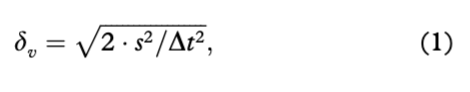
where s is the horizontal accuracy of the position and Δt is the interpolation interval. The accuracy of daily and hourly ice velocity is therefore 0.0003 and 0.006 m s−1, respectively.
To characterize the frequency-domain signal of ice velocity, we applied Fourier analysis using a fast Fourier transformation algorithm for normalized hourly velocities of buoys A, B and 2010A. Normalized velocities allow a better comparison among the frequency-domain signals, even when the absolute magnitude of ice velocity may change along the trajectory and among buoys. The normalized velocities were obtained by scaling the absolute values with the average values of a three-day sliding temporal window. The three-day sliding window was chosen as it suppresses the low-frequency signals from synoptic to seasonal scales and focuses on signals from hourly to daily. Data from buoy C were not used for frequency-domain analysis because of its low sampling frequency. The frequency of inertial oscillation depends on the latitude of the particle:
where f0 is the inertial frequency, with an unit of cycle day−1, Ω is the Earth’ rotation rate (1.002736 cycles day−1) and θ is the latitude. The inertial frequency ranges from 2.01 to 1.98 cycles day−1 between 90° and 80°N. Rotary spectra calculated from sea-ice velocity vector using complex Fourier analysis were used to distinguish signals of inertial and tidal origin, both of which have an almost identical frequency close to two cycles day−1 in the Arctic Ocean. According to Gimber, Marsan et al. (2012), the complex Fourier transformation is defined as
where N and Δt are the number and temporal interval of velocity samples, t0 and tend are the start and end of the temporal window, ux and uy are zonal and meridional ice speed at t+0.5Δt and ω is the angular frequency.
Assuming that sea ice can be represented as a homogeneous continuum, position measured by buoy arrays can be used to derive the divergence/convergence rate (D), shear rate (S) as well as the magnitude of the total deformation rate (ɛ) of sea ice, calculated as the square root of D and S (Herman & Glowacki 2012). As the buoys A–C formed a triangle for most of their joint deployment, we use their position data to derive sea-ice deformation. However, as the buoys A and C remained in close proximity, while buoy B moved further away, the derived deformation rate exhibited large uncertainty. Given this configuration, and following Heil et al. (2008), divergence/convergence of the ice field was approximated by the changes in distance among A–C, hence dominated by mesoscale drivers.
An independent data set was compiled to derive a broader picture of the long-term, seasonal and spatial changes in ice kinematics for the Arctic outflow region. This data set consisted of positions collected by 42 ice-tethered buoys, deployed between 1979 and 2011 and drifting between 88° and 80°N in the section from 60°W to 60°E. That included 38 buoys archived by the IABP combined with data from four 2010 buoys described above. Daily ice velocities, averaged over one-degree zones from 88° to 80°N for all buoys and all years, were used to estimate the seasonal and meridional variability. The MC of buoy trajectories (Heil et al. 2008) was used to assess the effective ice advection, which in turn affects the residence time of sea ice within the Arctic Ocean. Monthly MC was defined as the ratio of the cumulative distance along the trajectory determined by daily positions to the net displacement over one month.
Six-hourly data of 10-m wind speed and air temperature from the NCEP/NCAR Reanalysis 2 (Kanamitsu et al. 2002) were used to ascertain the local atmospheric forcing for the ice-tethered buoys. Sea-ice concentration derived from daily AMSR-E brightness temperatures (Spreen et al. 2008) was used to determine local ice condition for the 2010 buoys, noting that north of 88°N AMSR-E data are not available. Both data sets were bilinearly interpolated to the six-hourly positions of the buoys. The monthly NCEP/NCAR Reanalysis 2 SLP data above 70°N from 1979 to 2011 were used to derive the empirical orthogonal function modes. The AO and the DA correspond to the first and second leading modes of the empirical orthogonal function, respectively (Wang & Ikeda 2000; Wu et al. 2006). Here we analysed the empirical relationships between ice kinematic characteristics and monthly AO/DA indices obtained from the same time to explore the responses of ice drift to atmospheric circulation.
Results
Results derived from the buoys deployed in 2010
Operational history of buoys
After the deployments, driven by the TDS all buoys drifted from the central Arctic Ocean, through Fram Strait into the Greenland Sea (Fig. 1). Because of an unusual atmospheric circulation pattern bringing a warm air mass over the Arctic Ocean during August 2010, a distinctly transpolar ice melt occurred late summer 2010, from the central Arctic Ocean into northern Fram Strait (Kawaguchi et al. 2012). This resulted in relatively low ice concentration where the buoys A–C were deployed (Lei et al. 2012) and over the summer section of IMB 2010A’s track. Upon deployment, the sites of buoys A–C encountered ice melt with surface air temperatures (Ta) close to or above the freezing point. From mid-September 2010 onwards, the daily average Ta remained below 0°C through the entire life of buoy B, except for few episodic warm events. For buoys A and C, Ta rose above 0°C again in late May 2011. Thermistor chain measurements taken by buoy C demonstrated that thermodynamic ice growth occurred from early October 2010 to mid-May 2011. At the IMB 2010A site, Ta increased continuously from April to mid-June 2010, then fluctuated around 0°C until late August 2010, when it decreased gradually as winter approached. The operational lives of buoys A–C and IMB 2010A ended in May 2011, March 2011, July 2011 and December 2010, respectively, coinciding with their drift into the MIZ.
Sea-ice velocity
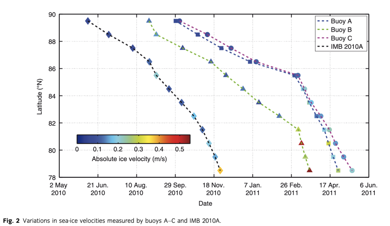
The six-hourly magnitude of buoy-derived ice velocity ranged from 0.01 to 0.64 m s−1 and increased as the ice moved into the Fram Strait. Mean ice velocity (0.15±0.12 m s−1) here was about twice the average ice velocity for the entire Arctic Ocean (Zhang et al. 2012). Generally less than 0.2 m s−1, the absolute zonal velocities were much smaller than the meridional velocities. The mean ratio between meridional and zonal velocities ranged from 1.14 to 1.64. Once the buoys had advanced into the Fram Strait (82° to 78°N), these ratios increased markedly, with mean values of 3.14, 2.34, 1.50 and 2.13 for buoys A–C and IMB 2010A, respectively. In contrast to buoys A, B and IMB 2010A, which traversed the eastern edge of the Fram Strait and subsequently entered into the MIZ, buoy C drifted further to the west. From there it merged into the East Greenland Current, where it encountered compact sea ice.
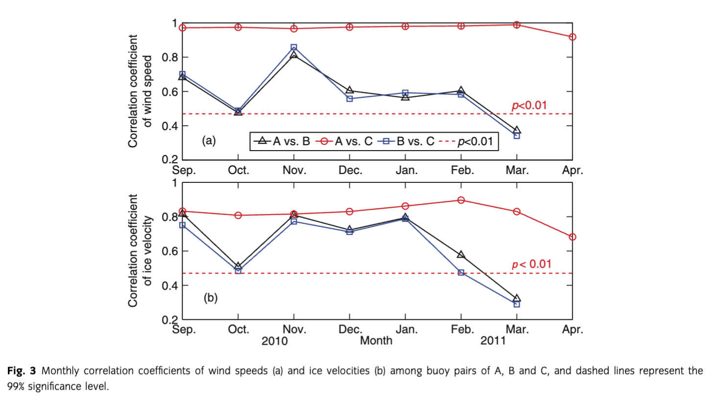
Because buoys A and C remained close to each other while north of 81°N, with a separation of 34–62 km, their mean velocities traced each other well except while moving between 84° and 83°N (Fig. 2). Monthly correlation coefficients of ice and wind speed of A and C remained high (above 0.9; P<0.01; Fig. 3). Their divergence in mean velocity was noted between 84° and 83°N (Fig. 3), which was associated with the buoys being exposed to different wind streams during a cyclone event. Buoy C was subject to an easterly surface wind and, consequently, its trajectory was more meandrous than that of buoy A. Once south of 81°N, buoy C progressed into an area of higher ice concentration and experienced less ocean-derived acceleration than buoy A.
Between 90° and 88°N buoy B was exposed to nearly double the wind speed as buoys A and C. Consequently, it moved at about 1.5–1.9 times their rate during October 2010 (Fig. 3). Between 88° and 85°N, the velocity of buoy B was close to those of A and C; however, between 85° and 83°N, buoy B slowed compared to A and C. This was likely related to the buoys moving in different wind regimes associated with a meso-scale cyclone, at times diverting buoy B into a northerly wind regime, while buoys A and C almost exclusively experienced southerlies. South of 82°N, the velocity of buoy B exceeded those of A and C, associated with its drift within the eastern section of the Fram Strait. IMB 2010A also clearly accelerated as it moved from the central Arctic Ocean into Fram Strait.
Responses to surface wind
Statistical relationships between sea-ice drift and surface wind speed based on six-hourly data are summarized in Table 2. North of 84°N, the ice drift speed was 1.6–2.2% of surface wind speed. The ratios increased markedly as the buoys drifted southward, to 1.9–3.0% at 80°–84°N and finally to 3.3–8.8% south of 80°N, which is larger than any results obtained from other Arctic regions. The initial increase was associated with increasing magnitude in wind speed, while the increased magnitude of the southward oceanic surface current was the likely driver to the high ratio through Fram Strait. The correlation coefficients between ice drift and surface wind speed north of Fram Strait were always larger than in Fram Strait, except for IMB 2010A. North of 80°N, the correlation coefficient at IMB 2010A was relatively low because of lower wind speeds at this buoy. The different response of ice drift at IMB 2010A to wind forcing highlights the seasonality of the wind regime.
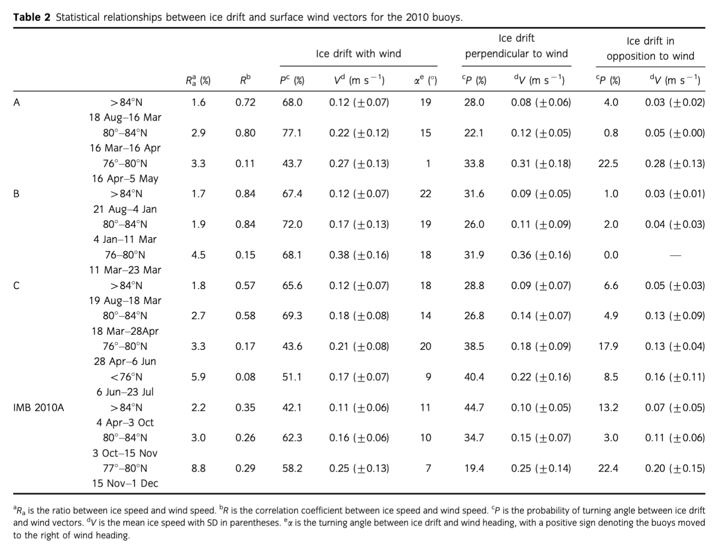
Ice drift can be classified by the absolute value of the turning angle between the ice-drift vector and the wind heading, following Vihma et al. (1996). Angles within 45° were assigned as “with wind heading”; angles between 45° and 135° as “perpendicular to wind heading”; and angles larger than 135° as “against wind heading.” North of Fram Strait, the majority of ice drift (42.1–82.4%) was in the direction of the wind. In Fram Strait, the relatively intense surface oceanic current dominated over the wind forcing, giving rise to a persistent southward ice drift, irrespective of the wind direction. In the case defined as “with wind heading,” the turning angle between ice drift and wind heading ranged from 10° to 22° north of Fram Strait. This range was close to those obtained in the Arctic TDS region during 2007–09 (5°–18°; Haller et al. 2014). As expected, the ice speed with wind heading exceeded that perpendicular to or against the wind heading.
Illustrated by buoy A, there was no dominant wind direction during October 2010, December 2010 and January 2011, which resulted in a relatively broad directional distribution of the ice vectors (Fig. 4). In November 2010 and March 2011, the ice vectors remained within a narrow range around 20° to the right of the wind in agreement with a tight wind heading. Consequently, the drift trajectory was more streamlined. During February 2011, the dominant wind heading ranged from north to north-west, opposing the direction of the TDS. This wind regime gave rise to two dominant ice-drift directions. Overall, the net displacement of buoy A was only 16 km during all of February 2011.
Inertial oscillation
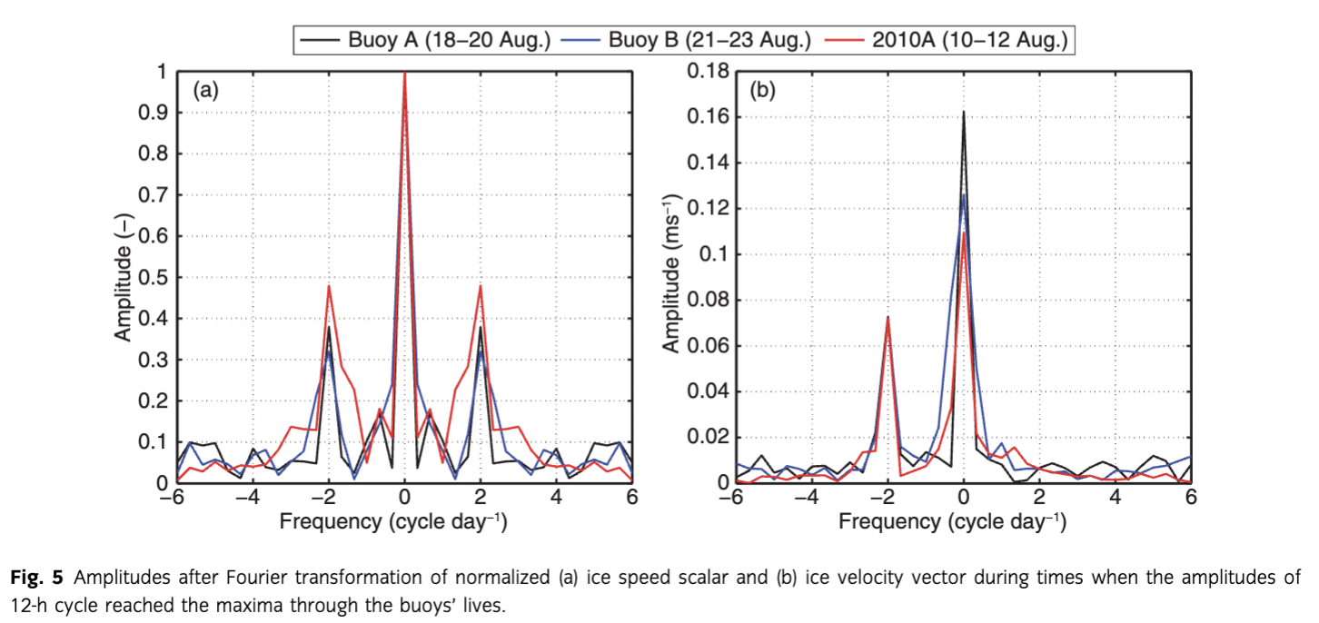
Based on the Fourier transformation, energy variance in the normalized sea-ice speed scalar was dominated by frequencies lower than 1.0 cycle day−1 and exhibited a clear secondary maximum at semidiurnal frequencies at about 2.0 cycles day−1 (Fig. 5a). The motion amplitudes of sea-ice velocities after the complex Fourier transformation show an asymmetrical pattern, with a distinct peak at the frequency of about −2 cycles day−1 (Fig. 5b), implying an identical clockwise oscillation (Heil et al. 2008; Gimbert, Marsan et al. 2012). The monotone oscillations of the buoys can be discerned from their tracks (Fig. 6). This semi-diurnal signal was therefore largely due to the inertial response.
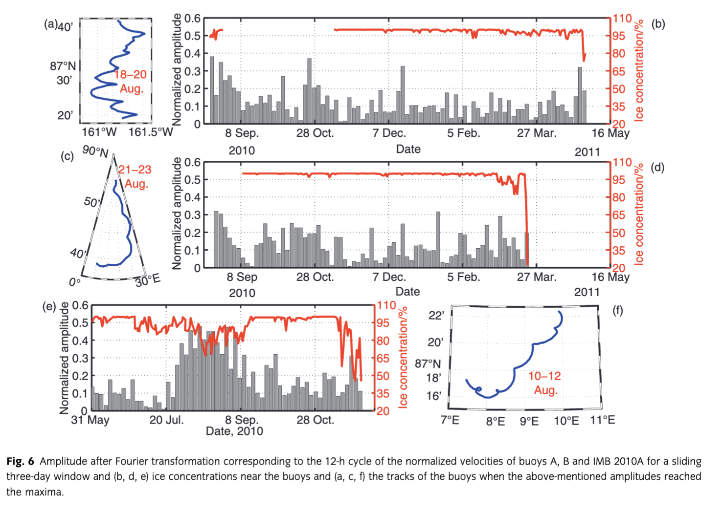
The magnitudes of the peak energy for the semi-diurnal frequency varied seasonally. For all buoys, the amplitudes of 12-h cycle reached the maxima in the summer time, that is, during 18–20, 20–23 and 10–12 August 2010 for the buoys A, B and IMB 2010A, respectively. For buoys A and B, semi-diurnal variability was observed distinctly from August to September 2010 (Fig. 6a–d). The inertially induced ice movement was damped with the advent of winter as ice concentration and internal stress increased. Once buoys A and B drifted into the MIZ, where the ice concentration rapidly decreased, the normalized amplitude at semi-diurnal frequencies increased slightly. IMB 2010A survived the summer within 88°–84°N. From late July onwards, the ice concentration near IMB 2010A decreased rapidly to a minimum of 65% on 15 August 2010. In consequence, the normalized velocity amplitudes at semi-diurnal frequencies increased markedly and persisted because of relatively low stress among the floes until ice concentration increased from mid-September onwards (Fig. 6e). This corroborates the results obtained from pan-Arctic analysis by Gimbert, Marsan et al. (2012), who also found that the sea-ice inertial response was strongest during the melting season. When IMB 2010A finally drifted into the MIZ, the velocity amplitude also increased slightly.
Sea-ice deformation
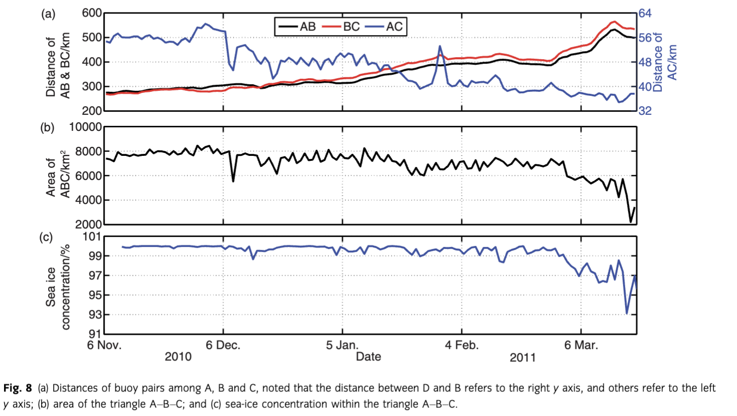
Initially, buoys A–C formed an isosceles triangle (Fig. 7). The area of the triangle remained stable prior to the end of February 2011. From the late December 2010 to late March 2011, once buoy B was south of 84°N and accelerated, the triangle ABC deformed. Around the same time, the base of the triangle shrunk slightly as buoys A and C converged as they approached Fram Strait (Fig. 8a). During March 2011, the area enclosed by the three buoys reduced to about 10% of the initial size due to a shear driven by an accelerated southward drift of buoy B. Generally, in Fram Strait, sea-ice convergence was induced by differential ice motion in zonal direction, while ice divergence arose from differential ice motion in the meridional direction. Overall, lead creation during divergence and lead closure during convergence balanced each other, as seen by the near-constant ice concentration within the triangle enclosed by ABC, which was reduced only once buoy B transited into the MIZ (Fig. 8c).

Ice drift derived using data from 1979 to 2011
Seasonal and spatial changes in sea-ice drift
Using drift data acquired between 88° and 80°N, and 60°W and 60°E, from the IABP archive and the buoys operating in 2010, irrespective of the year, the full picture of seasonal and spatial changes in sea-ice velocity can be obtained (Fig. 9). The relatively homogeneous distribution of time when the buoy data were available ensured the validity of the interpolation. Comparisons between the results derived from all buoys from 1979 to 2011 and those from the buoys in 2010 show that the ice speed in 2010 was slightly higher than the long-term average, but the discrepancy was not significant because their averages ±1 SD overlap for all latitudinal zones (Fig. 9d). Thus, 2010 can be considered a representative year relative for the 1979–2011 climatology with view to ice motion in the Arctic outflow region. The annual mean derived from the 1979–2011 data in 81–80°N of 0.18 m s−1 was about double that in 88–84°N of 0.08–0.10 m s−1 (Fig. 9d). These values were close to those obtained from a buoy array operating in the Arctic outflow region during 2007–09, given by Haller et al. (2014). They obtained the ice velocities of 0.08 m s−1 north of 85°N and 0.21 m s−1 in Fram Strait.
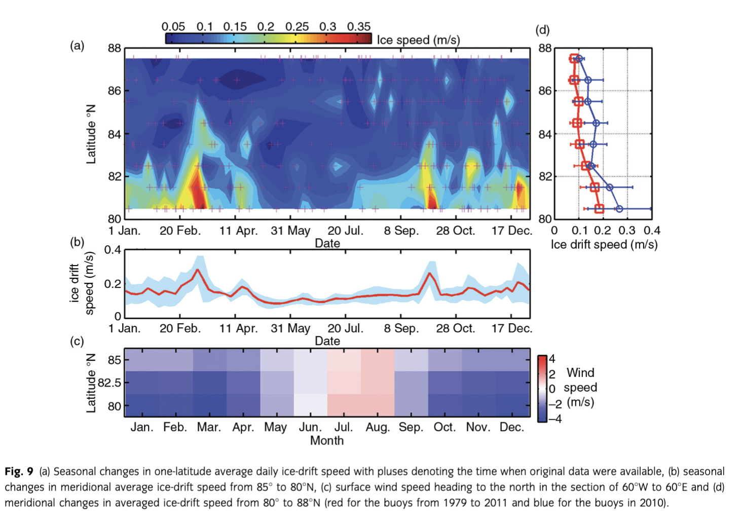
Distinct increases in both the magnitude and standard deviation of the annual mean ice velocity derived from the 1979 to 2011 data occurred from 84° to 80°N (Fig. 9d). The southward increase in the standard deviation can be attributed to the enhanced seasonal amplitude of ice velocity south of 84°N. Sea-ice speed increased from September to the following May (Fig. 9b). This seasonal pattern was related to the seasonality of surface wind. From September to May, the surface wind in the region was directed to the south, and the speed was relatively high from October to March, likely enhancing the TDS and increasing the southward ice velocity. Contrarily, during summer (June to August), the direction of the winds almost reversed against the dominant direction of TDS. Ice velocity was therefore relatively low during this time. For the buoys in 2010, the relatively slow drift of IMB 2010A compared with the buoys A–C was consistent with this seasonality (Fig. 2). Associated with relatively high ice concentration in winter, the seasonal changes in sea-ice area outflow through Fram Strait can be markedly enhanced. This explains the low contribution from June to September, accounting only about 13%, to the annual sea-ice area outflow through Fram Strait (Kwok 2009).
Long-term changes in sea-ice drift and responses to atmospheric circulation
Based on the long-term data set between 1979 and 2011, the mean travel time of sea ice from 88° to 80°N in the Arctic section of 60° to 60°E was 183 (±50) days (Fig. 10a). The mean travel time of the 2010 buoys was 154 (±29) days, which was shorter than the long-term average, but within the 1 SD of the long-term average. This again indicates that 2010 was a representative year. The linear regression shows that the long-term trend in the ice travel time from 1979 to 2011 was -0.05 days decade−1. However, this long-term trend was not statistically significant even at the 95% confidence level. Contrarily, the travel time shows high year-to-year variability, with the maximum roughly four times the minimum, because sea-ice export was highly promoted (restricted) during positive (negative) DA (Wang et al. 2009). About 31% of the variations in ice travel time from 88° to 80°N can be explained by the monthly DA index at the 99.9% significance level (Fig. 10b). The mean ice travel time in the positive regime of DA was 157 days (27 records), relative to 218 days in the negative regime of DA (15 records).
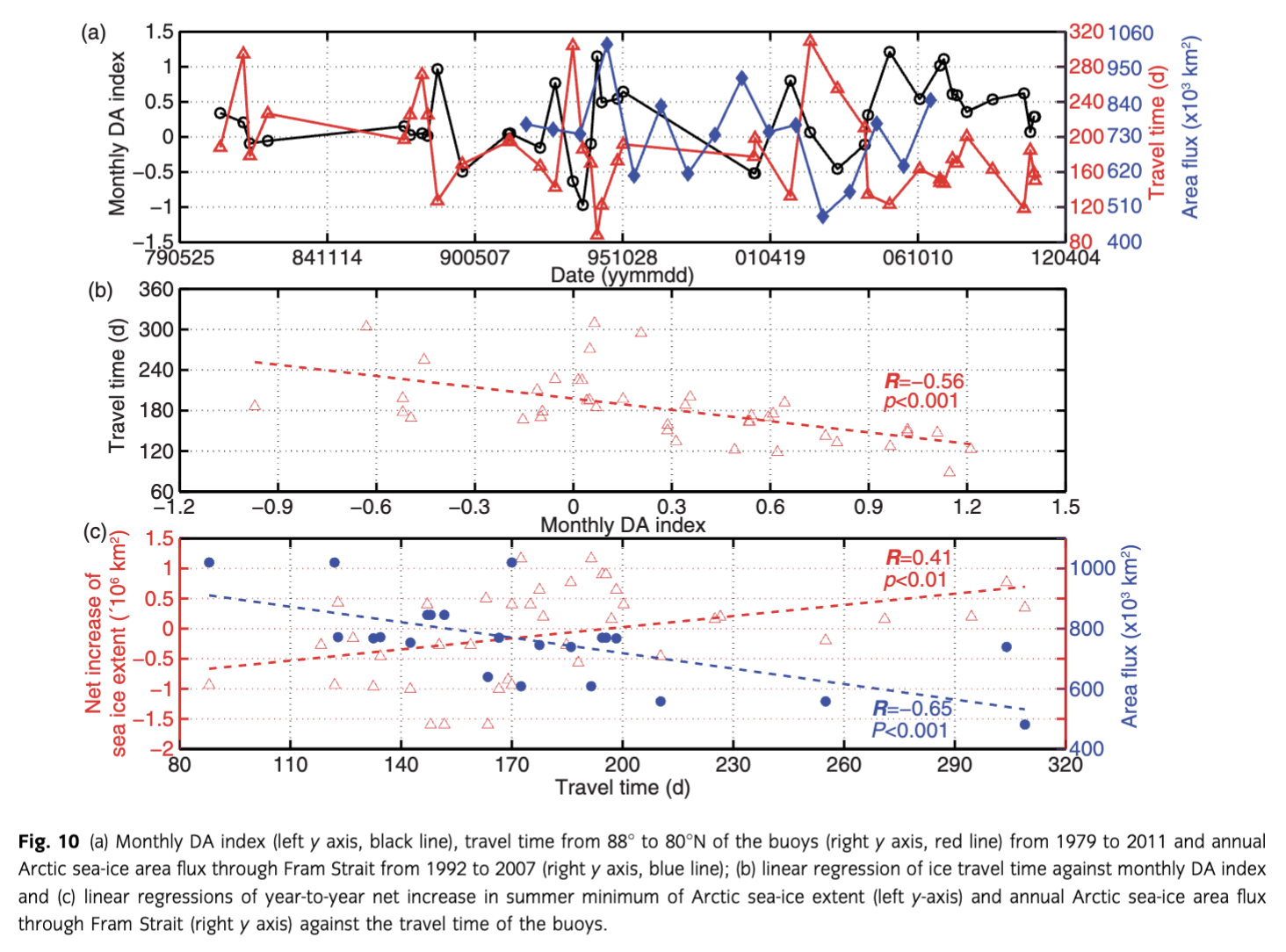
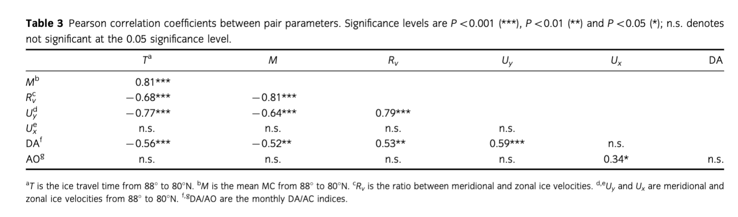
Using Pearson correlation analysis, we found that higher DA index coincided with relatively large meridional ice velocities (P<0.001; (Table 3), which was associated with a relatively small MC of ice drift (P<0.01). A strong positive (negative) phase of the AO was associated with a relatively large zonal cyclonic (anticyclonic) surface wind anomaly (Proshutinsky & Johnson 1997). There was a significant relationship between the AO and zonal ice velocity (P<0.05). However, as the ice travel time was largely dependent on meridional ice velocity ( P<0.001), the relationship between the AO index and ice travel time was statistically insignificant even at the 95% confidence level.
To explore the regional dependence of the relationship between the MC of ice drift and the DA index, we plotted all MCs against the latitudes and the monthly DA indices regardless of the year (Fig. 11). We found a spatial boundary at about 82°N. North of this latitude, the dependence of the MC on the DA index was stronger and both correlated well (R=0.41, P<0.001). In the high positive DA phase (>1.0) north of 82°N, the mean MC was 1.4 and the ice trajectories were more direct. In contrast, in the high negative phase of the DA (<−1.0), the mean MC was 4.3 and the ice drift trajectories were more meandering. For the neutral DA from −1.0 to 1.0, the mean MC was 1.9. South of 82°N, the meridional ice advection was more direct (mean MC of 1.3), regardless of the magnitude or phase of the DA index. This can be attributed to the marked increase in meridional ice velocity (Fig. 9d) due to direct forcing by the relatively fast surface oceanic current through Fram Strait.

To explore the relationship between the intensity of TDS and the decline of Arctic sea ice, we combined our data with results of the annual sea-ice area outflow through Fram Strait from 1992 to 2007 given by Kwok (2009) and calculated the year-to-year net change of summer minimum Arctic sea-ice extent. The net change of Arctic summer sea-ice extent was defined as the deviation between minimum Arctic sea-ice extents from a given year to the previous one. We found that a stronger TDS (shorter ice travel time from the central Arctic to Fram Strait) was associated with an increased sea-ice area outflow through Fram Strait (R=0.65, P<0.001) and a decline in Arctic summer sea-ice extent (R=0.41, P<0.01). For the extreme years of 1994–95, when the sea-ice area outflow through Fram Strait reached its maximum for 1992–2007, the mean monthly DA index and ice travel time from 88° to 80°N (obtained from three buoys) were 0.7 and 128 days, respectively. Consequently, the annual minimum Arctic sea-ice extent in September 1995 reached a record minimum since 1979. Relative to the 1994 summer, the net loss of annual minimum Arctic sea-ice extent in 1995 was 0.94×10⁶ km2. Contrarily, in 2002–03, when the sea-ice area outflow through the Fram Strait reached minimum for 1992–2007, the monthly DA index and mean ice travel time (obtained from two buoys) were −0.2 and 282 days, respectively. The net increase of annual minimum Arctic sea-ice extent in 2003 relative to 2002 was 0.35×10⁶ km2. Thereafter, the annual minimum sea-ice extent reached a record minimum again in the 2005 and 2007 summers. The mean travel times were 129 days (obtained from two buoys) and 158 days (obtained from four buoys), during 2004–05 and 2006–07, respectively. Both were clearly less than the long-term average (183 days) from 1979 to 2011. The persistent positive polarity of the DA since 2005, with a mean monthly DA index of 0.62 (±0.35), might give rise to the relatively short travel time of the floes from the central Arctic Ocean to Fram Strait, averaging 156 (±22) days. All years from 2005 to 2011 exhibited ice export faster than the long-term mean from 1979 to 2011, with only one exception (2008; 203 days), when the summer sea-ice extent showed a large recovery relative to the 2007 minimum. This suggests that the high ice outflow through Fram Strait played a significant role to accelerate the decline of the Arctic sea ice during recent years. However, the state since 2005 cannot be defined as a new normal, as similar high ice outflow rates were also observed in previous years, for example in the late 1980s and the mid-1990s.
Discussion and conclusions
Over an operational lifetime of 7–11 months from the Arctic outflow region into Fram Strait, six-hourly ice velocities derived from four buoys deployed in 2010 ranged from 0.01 to 0.64 m s−1 with an average of 0.15 (±0.12) m s−1. Daily ice velocities were slightly reduced to 0.13 (±0.09) m s−1 because of sub-diurnal meandering. Their travel time from 88° to 80°N was 154 (±29) days. While the long-term averages of daily ice velocities and travel time in Arctic outflow region (88°–80°N) from 1979 to 2011 were 0.10 (±0.08) m s−1 and 183 (±50) days, respectively. This implies that ice drift in this region for 2010–11 had increased slightly compared to the previous three decades, but still a normal state.
We measured a mean ice velocity in the Arctic outflow region about twice the Arctic Ocean average (Zhang et al. 2012). The data from 1979 to 2011 do not show any statistically significant long-term trend at the 95% significance level. Based on the comparison with the drift of the Norwegian vessel Fram 100 years ago, Gascard et al. (2008) and Haller et al. (2014) declared that the TDS has roughly doubled during 2007–09. However, the 1979–2011 data used here show that the relatively rapid TDS after 2005 cannot be defined as a new normal instead being a transient characteristic of the system, as similar high ice outflow rates were also observed in the late 1980s and the mid-1990s.
The strength of sea-ice outflow from the central Arctic Ocean to Fram Strait can be partially explained by the polarity of the DA (31%). The persistent positive phase of the DA since 2005 was associated with the relatively short travel time of sea ice, and consequently the accelerated decline of summer Arctic sea ice in recent years. We found a significant relationship (R=0.41, P<0.01) between sea-ice travel time from the central Arctic Ocean to Fram Strait and the year-to-year variability in minimum Arctic sea-ice extent. This lends further credibility to a conclusion that the TDS is a crucial factor determining the changes in Arctic sea ice (e.g., Kwok 2009; Wang et al. 2009; Wang et al. 2014).
North of Fram Strait, ice drift was closely coupled to the surface wind forcing, as seen by the strong correlation between ice velocity and wind speed, and a high probability of ice drifting with the wind. The impact on ice drift by the DA-derived anomalous meridional wind was therefore stronger in the region north of 82°N. A negative DA resulted in a wind direction against the TDS, and consequently increased the MC of the ice drift, and vice versa, during the positive phase of the DA. Once the ice had drifted towards and into Fram Strait, ice velocities increased markedly (about two to three times), due to the increase of the surface ocean current. This reduced response of ice drift to DA was associated with a decrease in ice meandering through Fram Strait. Sea-ice deformation also increased markedly as the floes congregated and drifted rapidly through Fram Strait. Deformation was characterized by meridional divergence and zonal convergence.
We suggest that south of 85°N, the distinct seasonal signal in the meridional wind velocity could possibly be linked to the seasonal pattern of Arctic sea-ice export through Fram Strait. In this region, the sea-ice velocity was relatively large from September to the following May. However, for two sub-data sets: six cases drifting from 84° to 80°N during June to August, and 26 cases during September to the following May, their average travel times from 88° to 80°N were 182±52 and 177±46 days, respectively. The difference was much less than 1 SD for both data sets. We therefore argue that interannual variability in ice travel time from the central Arctic Ocean to Fram Strait exceeded the seasonal change.
During summer, ice velocities exhibited a strong semi-diurnal signal. The result after the complex Fourier transformation of ice velocity indicates that this semi-diurnal signal was largely due to enhanced inertial response when the sea ice was less concentrated and there was less cohesion among the floes. In summer, the ratio of ice speed to wind speed was also larger, because of the enhanced free motion of floes. As winter approached, this semi-diurnal signal was quickly dampened by increased internal stress among the floes.
Acknowledgements
This work was financially supported by grants from the National Natural Science Foundation of China (no. 41476170), the Chinese Polar Environment Comprehensive Investigation and Assessment Programs (no. CHINARE2015-04-03/04-04/03-01) and Marine Public Industry Research of China (no. 201205007). Sea-ice concentration was provided by the University of Bremen (www.iup.uni-bremen.de:8084/amsr/amsre.html). IABP and their contributors are thanked for sharing buoy data (www.iabp.apl.washington.edu/). PH was supported under an Australian Antarctic Science grant (no. 4472) and by the Australian Government’s Cooperative Research Centres Programme through the Antarctic Climate and Ecosystems Cooperative Research Centre. JW was supported by the National Oceanic and Atmospheric Administration Office of Arctic Research (grant no. 1755). We also thank the anonymous reviewers for their comments, and S. Lake and C. Darnell for editing the manuscript.
References
- Comiso J.C. 2012. Large decadal decline of the Arctic multiyear ice cover. Journal of Climate 25, 1176–1193. Publisher Full Text
- Cox K.A., Stanford J.D., McVicar A.J., Rohling E.J., Heywood K.J., Bacon S., Bolshaw M., Dodd P. A., De la Rosa S. & Wilkinson D. 2010. Interannual variability of Arctic sea ice export into the East Greenland Current. Journal of Geophysical Research—Oceans 115, C12063, doi: http://dx.doi.org/10.1029/2010JC006227 Publisher Full Text
- Gascard J.-C., Festy J., Le Goff H., Weber M., Brümmer B., Offermann M., Doble M., Wadhams P., Forsberg R., Hanson S., Skourup H., Gerland S., Nicolaus M., Metaxian J.-P., Grangeon J., Haapala J., Rinne E., Haas C., Heygster G., Jacobson E., Palo T., Wilkinson J., Kaleschke L., Claffey K., Elder B. & Bottenheim J. 2008. Exploring Arctic transpolar drift during dramatic sea ice retreat. EOS, Transactions of the American Geophysical Union 89, 21–28. Publisher Full Text
- Gimbert F., Jourdain N.C., Marsan D., Weiss J. & Barnier B. 2012. Recent mechanical weakening of the Arctic sea ice cover as revealed from larger inertial oscillations. Journal of Geophysical Research—Oceans 117, C00J12, doi: http://dx.doi.org/10.1029/2011JC007633
- Gimbert F., Marsan D., Weiss J., Jourdain N.C. & Barnier B. 2012. Sea ice inertial oscillations in the Arctic Basin. The Cryosphere 6, 1187–1201. Publisher Full Text
- Hakkinen S., Proshutinsky A. & Ashik I. 2008. Sea ice drift in the Arctic since the 1950s. Geophysical Research Letters 35, L19704, doi: http://dx.doi.org/10.1029/2008GL034791 Publisher Full Text
- Haller M., Brümmer B. & Müller G. 2014. Atmosphere–ice forcing in the transpolar drift stream: results from the DAMOCLES ice-buoy campaigns 2007–2009. The Cryosphere 8, 275–288. Publisher Full Text
- Heil P. & Hibler W.D., III. 2002. Modeling the high-frequency component of Arctic sea ice drift and deformation. Journal of Physical Oceanography 32, 3039–3057. Publisher Full Text
- Heil P., Hutchings J.K., Worby A.P., Johansson M., Launiainen J., Haas C. & Hibler W.D., III. 2008. Tidal forcing on sea-ice drift and deformation in the western Weddell Sea in early Austral summer 2004. Deep-Sea Research Part II 55, 943–962. Publisher Full Text
- Herman A. & Glowacki O. 2012. Variability of sea ice deformation rates in the Arctic and their relationship with basin-scale wind forcing. The Cryosphere 6, 1553–1559. Publisher Full Text
- Hilmer M. & Jung T. 2000. Evidence for a recent change in the link between the North Atlantic oscillation and Arctic sea ice export. Geophysical Research Letters 27, 989–992. Publisher Full Text
- Kanamitsu M., Ebisuzaki W., Woollen J., Yang S., Hnilo J.J., Fiorino M. & Potter G.L. 2002. NCEP–DOE AMIP-II reanalysis (R-2). Bulletin of the American Meteorological Society 83, 1631–1643. Publisher Full Text
- Kawaguchi Y., Hutchings J.K., Kikuchi T., Morison J.H. & Krishfield R.A. 2012. Anomalous sea-ice reduction in the Eurasian Basin of the Arctic Ocean during summer 2010. Polar Science 6, 39–53. Publisher Full Text
- Kwok R. 2009. Outflow of Arctic Ocean sea ice into the Greenland and Barents seas: 1979–2007. Journal of Climate 22, 2438–2457. Publisher Full Text
- Kwok R., Spreen G. & Pang S. 2013. Arctic sea ice circulation and drift speed: decadal trends and ocean currents. Journal of Geophysical Research—Oceans 118, 2408–2425. Publisher Full Text
- Lei R., Zhang Z., Matero I., Cheng B., Li Q. & Huang W. 2012. Reflection and transmission of irradiance by snow and sea ice in the central Arctic Ocean in summer 2010. Polar Research 31, article no. 17325, doi: http://dx.doi.org/10.3402/polar.v31i0.17325 Publisher Full Text
- Leppäranta M. 2011. The drift of sea ice. Berlin: Springer Press.
- Maslanik J., Drobot S., Fowler C., Emery W. & Barry R. 2007. On the Arctic climate paradox and the continuing role of atmospheric circulation in affecting sea ice conditions. Geophysical Research Letters 34, L03711, doi: http://dx.doi.org/10.1029/2006GL028269
- Nghiem S.V., Rigor I.G., Perovich D.K., Clemente-Colon P., Weatherly J.W. & Neumann G. 2007. Rapid reduction of Arctic perennial sea ice. Geophysical Research Letters 34, L19504, doi: http://dx.doi.org/10.1029/2007GL031138 Publisher Full Text
- Parkinson C.L. & Comiso J.C. 2013. On the 2012 record low Arctic sea ice cover: combined impact of preconditioning and an August storm. Geophysical Research Letter 40, 1356–1361. Publisher Full Text
- Proshutinsky A.Y. & Johnson M.A. 1997. Two circulation regimes of the wind-driven Arctic Ocean. Journal of Geophysical Research—Oceans 102, 12493–12514. Publisher Full Text
- Rampal P., Weiss J. & Marsan D. 2009. Positive trend in the mean speed and deformation rate of Arctic sea ice, 1979–2007. Journal of Geophysical Research—Oceans 114, C05013, doi: http://dx.doi.org/10.1029/2008JC005066
- Rampal P., Weiss J., Marsan D., Lindsay R. & Stern H. 2008. Scaling properties of sea ice deformation from buoy dispersion analysis. Journal of Geophysical Research—Oceans 113, C03002, doi: http://dx.doi.org/10.1029/2007JC004143
- Rigor I.G., Wallace J.M. & Colony R.L. 2002. Response of sea ice to the Arctic oscillation. Journal of Climate 15, 2648–2663. Publisher Full Text
- Serreze M.C., Barrett A.P., Slater A.G., Woodgate R.A., Aagaard K., Lammers R.B., Steele M., Moritz R., Meredith M. & Lee C.M. 2006. The large-scale freshwater cycle of the Arctic. Journal of Geophysical Research—Oceans 111, C11010, doi: http://dx.doi.org/10.1029/2005JC003424 Publisher Full Text
- Spreen G., Kaleschke L. & Heygster G. 2008. Sea ice remote sensing using AMSR-E 89 GHz channels. Journal of Geophysical Research—Oceans 113, C02S03, doi: http://dx.doi.org/10.1029/2005JC003384
- Spreen G., Kwok R. & Menemenlis D. 2011. Trends in Arctic sea ice drift and role of wind forcing: 1992–2009. Geophysical Research Letters 38, L19501, doi: http://dx.doi.org/10.1029/2011GL048970 Publisher Full Text
- Stern H.L. & Lindsay R.W. 2009. Spatial scaling of Arctic sea ice deformation. Journal of Geophysical Research—Oceans 114, C10017, doi: http://dx.doi.org/10.1029/2009JC005380 Publisher Full Text
- Stouffer R.J., Yin J., Gregory J.M., Dixon K.W., Spelman M.J., Hurlin W., Weaver A.J., Eby M., Flato G.M., Hasumi H., Hu A., Jungclaus J.H., Kamenkovich I.V., Levermann A., Montoya M., Murakami S., Nawrath S., Oka A., Peltier W.R., Robitaille D.Y., Sokolov A., Vettoretti G. & Weber S.L. 2006. Investigating the causes of the response of the thermohaline circulation to past and future climate changes. Journal of Climate 19, 1365–1387. Publisher Full Text
- Timmermans M.-L., Proshutinsky A., Krishfield R.A., Perovich D.K., Richter-Menge J.A., Stanton T.P. & Toole J.M. 2011. Surface freshening in the Arctic Ocean’s Eurasian Basin: an apparent consequence of recent change in the wind-driven circulation. Journal of Geophysical Research—Oceans 116, C00D03, doi: http://dx.doi.org/10.1029/2011JC006975
- Tremblay L.-B. & Mysak L.A. 1997. Modeling sea ice as a granular material, including the dilatancy effect. Journal of Physical Oceanography 27, 2342–2360. Publisher Full Text
- Tsukernik M., Deser C., Alexander M. & Tomas R. 2010. Atmospheric forcing of Fram Strait sea ice export: a closer look. Climate Dynamics 35, 1349–1360. Publisher Full Text
- Vihma T., Launiainen J. & Uotila J. 1996. Weddell Sea ice drift: kinematics and wind forcing. Journal of Geophysical Research—Oceans 101, 18279–18296. Publisher Full Text
- Vihma T., Tisler P. & Uotila P. 2012. Atmospheric forcing on the drift of Arctic sea ice in 1989–2009. Geophysical Research Letters 39, L02501, doi: http://dx.doi.org/10.1029/2011GL050118 Publisher Full Text
- Wang J., Eicken H., Yu Y., Bai X., Zhang J., Hu H., Wang D.-R., Ikeda M., Mizobata K. & Overland J.E. 2014. Abrupt climate changes and emerging ice–ocean processes in the Pacific Arctic region and the Bering Sea. In J.M. Grebmeier & W. Maslowski (eds.): The Pacific Arctic region: ecosystem status and trends in a rapidly changing environment. Pp. 65–100. Dordrecht: Springer.
- Wang J. & Ikeda M. 2000. Arctic oscillation and Arctic sea-ice oscillation. Geophysical Research Letters 27, 1287–1290. Publisher Full Text
- Wang J., Zhang J., Watanabe E., Mizobata K., Ikeda M., Walsh J.E., Bai X. & Wu B. 2009. Is the dipole anomaly a major driver to record lows in the Arctic sea ice extent? Geophysical Research Letters 36, L05706, doi: http://dx.doi.org/10.1029/2008GL036706
- Wu B., Wang J. & Walsh J.E. 2006. Dipole anomaly in the winter Arctic atmosphere and its association with Arctic sea ice motion. Journal of Climate 19, 210–225. Publisher Full Text
- Zhang J., Lindsay R., Schweiger A. & Rigor I. 2012. Recent changes in the dynamic properties of declining Arctic sea ice: a model study. Geophysical Research Letters 39, L20503, doi: http://dx.doi.org/10.1029/2012GL053545
- Zhang J., Woodgate R. & Moritz R. 2010. Sea ice response to atmospheric and oceanic forcing in the Bering Sea. Journal of Physical Oceanography 40, 1729–1747. Publisher Full Text
Related Articles
Theodora Pados
Robert F. Spielhagen
Eva-Maria Nöthig
Astrid Bracher
Anja Engel
Katja Metfies
et al.
Christian Lydersen
Kit M. Kovacs
Jade Vaquie-Garcia
Espen Lydersen
et al.
Alexander Vetrov
Evgeny Romankevich
Walter N. Meier
Ge Peng
Donna J. Scott
Matt H. Savoie
et al.