This article is published under a Creative Commons license and not by the author of the article. So if you find any inaccuracies, you can correct them by updating the article.

Models in Science Education: Applications of Models in Learning and Teaching Science


Funda Ornek
Published: April 10, 2008
Latest article update: Dec. 29, 2022
This article is published under the license


Abstract
In this paper, I discussed different types of models in science education and applications of them in learning and teaching science in particular physics. Based on the literature, I categorized models as conceptual and mental models according to their characteristics. In addition to these models, there is another model called “physics model” by the physics-education community. And then, I discussed applications of these models for learning and teaching science particularly physics along with examples that can guide teachers and students in their science courses.
Keywords
Learning, Model-Based Learning, Science Education, Conceptual Development, Physics Education
INTRODUCTION
What is a model?
In a general sense, a model is a representation of a phenomenon, an object, or idea (Gilbert, 2000). In science, a model is the outcome of representing an object, phenomenon or idea (the target) with a more familiar one (the source) (Tregidgo & Ratcliffe, 2000). For example, one model of the structure of an atom (target) is the arrangement of planets orbiting the Sun (source) (Tregidgo & Ratcliffe, 2000).
The model can only relate to some properties of the target. Some aspects of the target must be excluded from the model (Driel & Verloop, 1999). For example, the solar system model of the atom models the nucleus surrounded by electrons but excludes the delocalization of electrons, among other aspects. With respect to physics, Hestenes (1996) describes a model as a representation of structure in a physical system and/or its properties. The system may consist of one or more material objects. A model refers to an individual system, though that individual may be an exemplar for a whole class of similar things.
Models in Science Education
There are different types of models in science education. To categorize them, we should look into what makes them be considered different. For this reason, we should understand the difference between conceptual and mental models. Conceptual models are devised as tools for the understanding or teaching of systems. In addition to this, conceptual models are external representations—socially constructed and shared—which are precise, complete and consistent with the shared scientific knowledge specially created to facilitate the comprehension or the teaching of the systems in the world (Greace & Moreira, 2000). On the other hand, mental models are what people really have in their heads and what guides their use of things (Norman, 1983). Buckley et al. (2004) also viewed mental models as internal, cognitive representations.
Based on the literature, conceptual models include mathematical models, computer models, and physical models which are discussed in the following sections. In addition to these models, there is another model called “physics model” by the physics- education community. Physics models will be discussed later.
Categories of Models
In this section, I will discuss mental models, conceptual models, and physics models respectively. Conceptual models are mathematical models, computer models, and physical models.
Mental Models
Mental models are psychological representations of real or imaginary situations. They occur in a person’s mind as that person perceives and conceptualizes the situations happening in the world (Franco & Colinvaux, 2000). Norman (1983) indicates that mental models are related to what people have in their heads and what guides them using these things in their minds. In order to understand mental models, their characteristics should be considered.
Mental models have a variety of features (Franco & Colinvaux, 2000). These are:
- Mental model: an generative.
- Mental model: involve tacit knowledge.
- Mental model: an synthetic
- Mental model: an restricted by world-view.
Before explaining each of these features, one example regarding mental models from Vosniadou and Brewer’s (1992) study, which probes elementary school
students’ understanding of the Earth, its shape, and the regions where people live, can be helpful for understanding mental models. In the study, students were asked some questions to find out their mental models of the Earth, its shape, and the regions where people live. During these interviews with students, they were also asked to use drawings. Some of the questions were “what is the shape of the Earth? If you were to walk for many days in a straight line where would you end up?” To answer these questions, students needed to refer their previous experience and knowledge to create their mental models.
According to the results of their study, various mental models were found as shown in Figure 1.
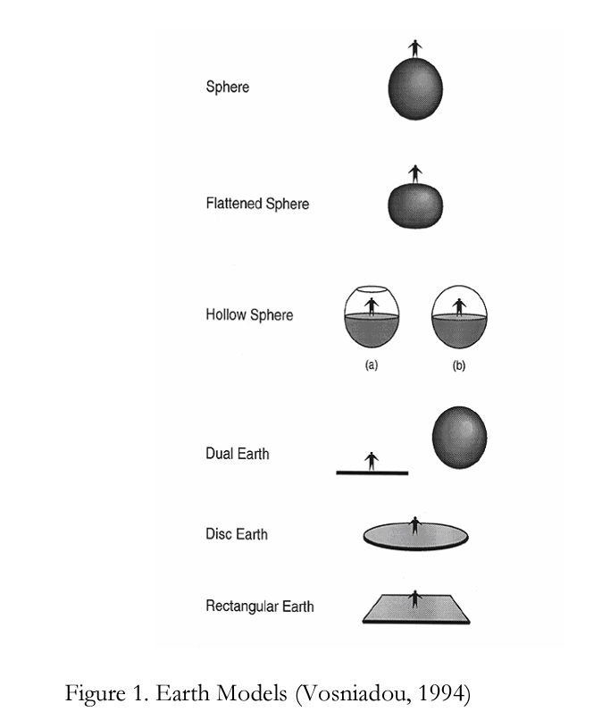
- The spherical Earth model: The earth is a sphere with people living all around it on the outside.
- The flattened sphere model: The earth is a sphere but flattened at the poles, or a thick pancake.
- The hollow sphere model: The earth is a hollow sphere with people living on flat ground inside it or it is made of two hemispheres, the lower one on which people live and the upper one with the sky like a dome.
- The dual Earth model: This includes two earths, a mund one up in the sky and aflat, solid and supported earth-the ground where people live.
- The disc Earth model: The earth presents same features as in the rectangular earth model; only difference is that the earth is shaped like a disc.
- The rectangular Earth model: The earth appears as a flat, solid, supported object shaped like a rectangle.
I will now go back to describing the features of mental models using these children’s models as examples.
- Mental models are generative (Franco & Colinvaux, 2000): This means that people or students can produce new information and make predictions while they are using mental models. For example, in Vosniadou and Brewer’s study, they asked questions such as “if you walked for many days in a straight line, where would you end up? Is there an end or an edge to the earth?” When students said “yes” for the latter question, the asked further questions such as “can you fall off that end or edge? Where would you fall?” These questions make students become creative because they cannot observe these phenomena. According to students’ earth models, for example, the disc, the rectangular, and the dual earth models show that earth has an edge or end from which people can fall off. Also, the hollow sphere model has an edge, however people live inside, and it is not possible for people to fall off (Vosniadou & Brewer, 1992).
- Mental models involve tacit knowledge (Franco & Colinvaux, 2000): The person who uses a mental model is not completely aware of some aspects of his or her mental models. In general, students have some presuppositions about physical or any other phenomena. These are really implicit. They are not conscious and people do not think about them, but rather they use them for reasoning. One example will explain this aspect of mental models. From Vosniadou and Brewer’s study (1994), in the disc and rectangular models of earth, students have presuppositions that the ground is flat. This presupposition is implicit, but it can be made explicit through their drawings.
- Mental models are synthetic (Franco & Colinvaux, 2000): Mental models are simplified representations of the target system which can be a phenomenon or event. That is, they cannot represent the complete phenomenon or event. What is meant by representation? A representation is never a complete reproduction of what is being represented but, requires conscious or unconscious selection of what aspects will be represented and what other aspects will be left out of the representation (Franco & Colinvaux, 2000). In order to develop a representation of a target, some aspects are isolated to make some kind of simplifications.
- Mental models are constrained by worldviews (Franco & Colinvaux, 2000): People develop and use mental models according to their beliefs. In other words, a set of limitations forms the possible mental models which people use. Above, students’ mental models about earth models formed and developed according to their presuppositions. For instance, students build the disc and a rectangular model of earth from their presupposition which is the earth is flat. Moreover, for the dual earth, hollow sphere, and flattened earth models, they had the presupposition which is the ground on which people live is flat, but earth is round. Therefore, the earth mental models according to students’ mental models are constrained by
presuppositions, also used as misconceptions (Franco & Colinvaux, 2000).
Conceptual Models
A conceptual model is an external representation created by teachers, or scientists that facilitates the comprehension or the teaching of systems or states of affairs in the world (Greca & More ire, 2000 and Wu et al., 1998). According to Norman (1983), conceptual models are external representations that are shared by a given community, and have their coherence with the scientific knowledge of that community. These external representations can be mathematical formulations, analogies, graphs, or material objects. An example of an object could be a water pump which is sometimes used to model a battery in an electric circuit. An analogy can be established between an atom and the solar system. The ideal gas model is a mathematical formulation (Greca & Moreire, 2000). To come to the point, we can say that conceptual models are simplified and idealized representations of real objects, phenomena, or situations.
Since mathematical models, computer models, and physical models are external representations, they will be discussed in the following sections under conceptual models.
Mathematical Models
A mathematical model is the use of mathematical language to describe the behavior of a system. That is, it is a description or summarization of important features of a real-world system or phenomenon in terms of symbols, equations, and numbers. Mathematical models are approximations. They do not always yield what is actually measured. A
simple example is "F=m*g". If we want to express the gravitational forces on a falling ball exactly, we must consider the force between each possible pair of atoms and sum the vectors. F=m*g yields a value that is close enough to use in most situations. F=m*g only works for millions of molecules (like a baseball) close to the surface of the Earth. It does not work for a single molecule because we need to consider interactions with other molecules.
Mathematics provides one of the powerful tools for modeling and solving problems in science and other areas. For instance, in chemistry, and physics, we use mathematical techniques to model situations and solve problems (Hodgson et al., 1999).
Burghes and Borrie (1979) described mathematical modeling as the way in which “real-world” problems are translated into mathematical models and also, how the results can be applied to the real-world situations. In other words, it is the application of mathematics to Science, Physics, and many other fields.
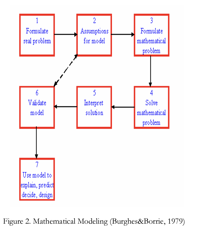
The process of mathematical modeling can be summarized in figure 2.
The left side (boxes 1, 6, and 7) represents the real-world. The right side (boxes 3 and 4) represents the mathematical-world. The middle part (boxes 2 and 5) represents the connection between the real and mathematical worlds. In the middle part, the problem is first simplified and converted into mathematical language and later, the mathematical solution is translated back into the real world.
Generally, in mathematical modeling, the setting up of the problem, qualitative validation, and qualitative prediction sections are important before starting to solve the problem.
Related to this explanation in terms of mathematical modeling, here is an example about how to use mathematical modeling to solve a physics problem. In this example, the way in which problems are translated into mathematical models and also, how the results can be applied to the real-world situations are shown (Burghes & Borrie, 1979).
Example: Critical angle for shot putters: A shot putter lays great emphasis on a smooth build up of speed across the throwing circle and this enables him to accelerate the shot in a straight line up to the point of release. But at what angle should he aim to release the shot, and does it make a significant difference to the distance thrown?
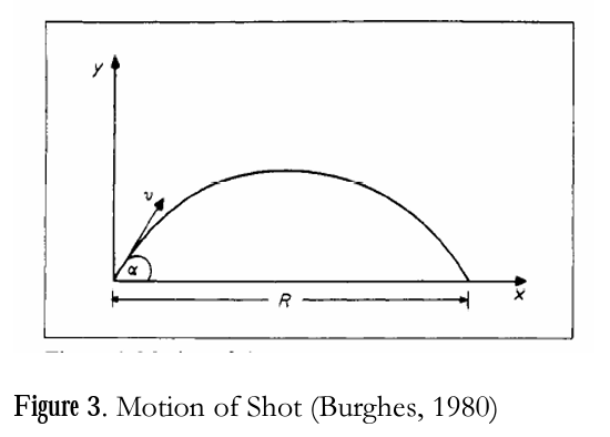
For an initial model, it can be assumed that the motion is two dimensional as shown in Figure 3.
We can suppose that the shot leaves with speed и at angle a to the horizontal, and assuming constant gravity and no resistive forces, we have the usual equations of motion which give the horizontal range as
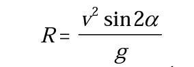
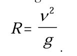
For maximum R, sin2a should be equal to 1 which gives the critical angle a=45. Therefore, for our mathematical model, the optimum projection angle is 45. So, the range becomes
Besides this, we made other assumptions. For example, we can assume that the shot can be considered as a “point” particle. We can neglect air resistance, also, we can assume that the shot is projected from the ground level y=0. Even though this model has some limitations, we can have some conclusions. For instance, the putter makes an error of the critical angle by 10%; therefore he/she throws it with 49.5 The range becomes
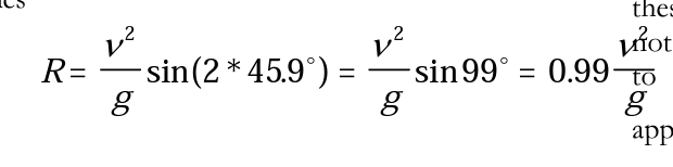
So, having the angle of 49.5 results in 1% decrease in the range. From this, we can conclude that the model says that critical angle is not significant. That is, its effect is not much. It is more significant that the putter would increase his/her projection speed. For example, when he/she increases 5% in speed which is going to increase from и to 1.05u, the range will increase 10%. According to the definition of Burghes and Borrie (1979), this example is a mathematical modeling because it shows the usage of the real-world problem —how to achieve the best throw- and translates it to a mathematical problem by formulation of a mathematical model. So, the shot putter had his best throw after this problem was solved by using mathematical model.
Interpretation about descriptive variables. Interpretation is critical for a model because without interpretation the equations of a model do not say anything. The equations are abstract by themselves.
Object variables: These are fundamental properties of objects. For instance, mass and charge are object variables for the electron. Moment of inertia and forms of shape and size are the object variables for the rigid body. So, we can say that the object variables are the fixed values for a specific object.
State variables'. These are fundamental properties which can vary with time. They are not fixed values like object values. For instance, position and velocity are state values for an object. State variables in one model can be object variables in another model. For example, although mass is a state variable in a model of rocket because it is changing with time, it is an object variable in other model such as particle models because it is constant.
Interaction variables: These represent the interaction of some external object such as the friction force, with the object being modeled. For example, in mechanics one of the interaction variables is the force vector. Work, potential energy, and torque are other interaction variables.
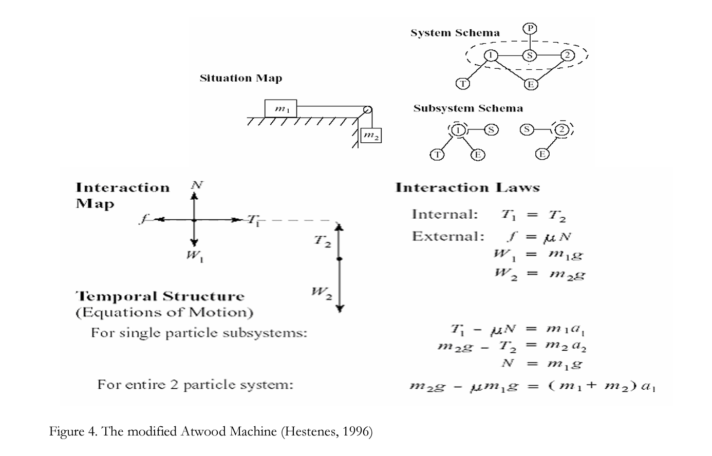
An example from Hestenes (1996) about a mathematical model in terms of mechanics in physics explains more explicitly what a mathematical model is according to him.
In Figure 4, the Situation Map shows a system which is composed of 2 objects, two masses ml and m2 connected by a massless string (S). These objects interact with external agents, the table (T), the earth (E), and the pulley (P) as indicated in System Schema. The descriptive variables are shown as the force vectors such as tensions on the strings, weights of masses, and masses in the Interaction Map. The equations of the model are shown in the temporal structure for the whole system of two objects and for each single object. The System Schema and Subsystem Schema specify the composition, environment, and connections of the system. The System Schema specifies a system which is composed of two objects connected by a string (S), earth (E), and pulley (P). The closed dotted lines are to separate the system from its environment. In the Interaction Laws, first, the forces on each object are represented by force diagrams. Second, magnitudes of the forces are specified by a set of Interaction (force) Laws. In the temporal structure part, equations of motion are written by using Newton’s Second Law F=ma for both two particle system and a single particle systems. The last part is the interpretation of the equations.
Computer Models
A computer model is a computer program which attempts to simulate the behavior of a particular system. In other words, a computer model is a computer program which is created by using a mathematical model to find analytical solutions to problems which enable the prediction of the behavior of the complex system from a set of parameters and initial conditions.
Computer models allow students to develop numerical models of the real world. The software is called a modeling system or simulation language (Holland, 1988). Such computer simulations make it possible for students to analyze complex systems. Sometimes, complex systems require really very sophisticated mathematics to analyze and they cannot be analyzed without computers (Chabay & Sherwood, 1999). Computer simulations may employ many representations such as pictures, two-dimensional or three-dimensional animations, graphs, vectors, and numerical data displays which are helpful in understanding the concepts (Sherer et al., 2000). These simulations can be either icon-oriented programs or programs written by the user. For example, java applets are icon-oriented programs in which students do not need to write the simulation programs, they just need to change parameters. In this situation, students can only analyze a model instead of creating their own models. An alternate software is the Vpython programming language which allows students to create their own models. Students are involved in writing and modifying programs if needed. The main purpose is to understand the phenomenon.
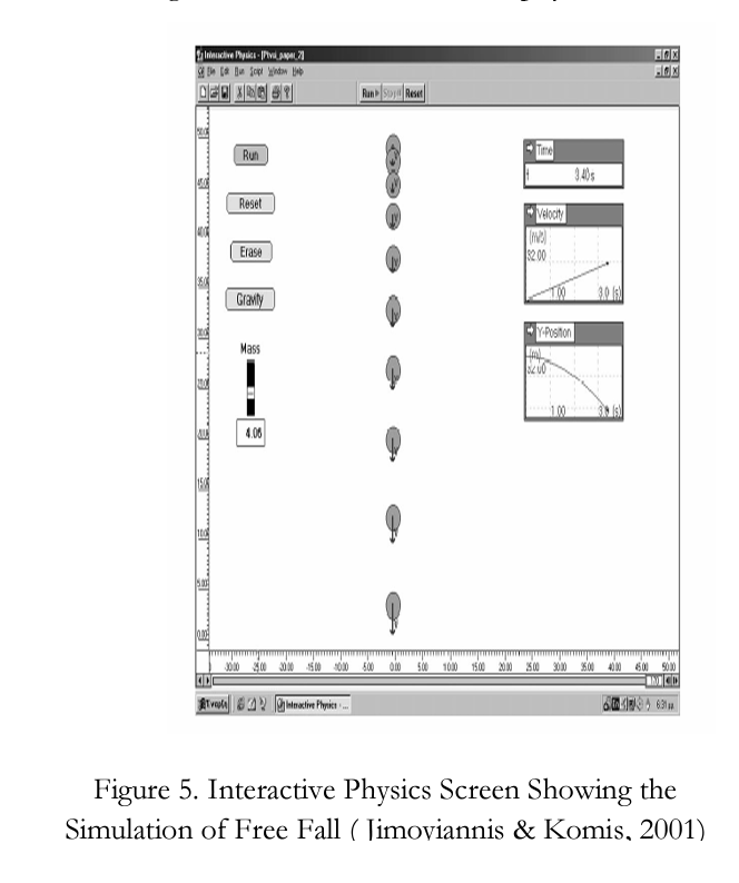
Here is an example of simulating Newtonian mechanics through an icon-oriented simulations program (Interactive Physics, Jimoyiannis & Komis, 2001). First, let me explain a little bit about the Interactive Physics software. It provides 2-D simulations with which students can simulate fundamental principles of Newtonian mechanics. Students do not need to do any programming. They simply enter the values of variables such as mass, or velocity. Simulations are produced by the system. Many physical quantities can be measured. Figure 5 shows the interactive physics screen that simulates a ball falling freely from a given height in the earth’s gravitational field. Students can experiment by changing the value of the parameters in the system, study the physical laws, make assumptions and predictions, and make conclusions from the stroboscopic representation of a kinematical phenomenon and the simultaneous display of the position and velocity. Students can repeat their experiments whenever they need to do so. Also, they can modify the mass of the sphere or hold the gravity constant. They can see the results on the computer screen and they can get the values of the position у and the velocity Vy of the moving object.
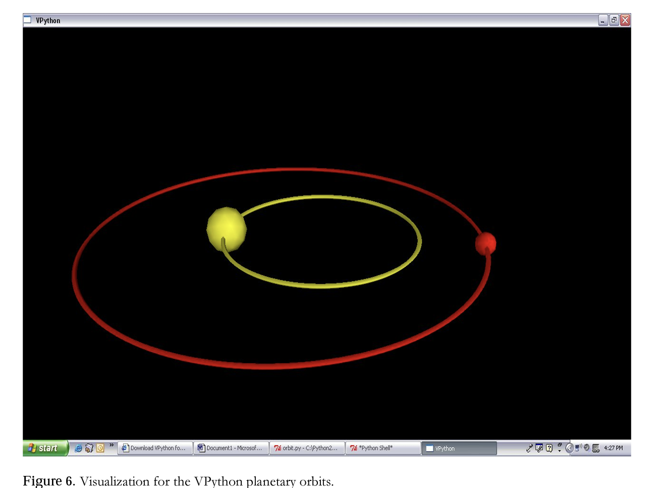
The other example related to computer simulation is to use software to create simulations in the VPython programming language. VPython makes students focus on the physics computations to obtain 3- D visualizations. Students can do true vector computations, which improves their understanding of the utility of vectors and vector notation. For example, students can study the motion of the earth in orbit around the sun by means of writing a program. Furthermore, students can study the motion of a planet around a star using the computer model of the Earth and Sun. The printout of the simulation is shown in the following Figure 6.
Figure 6 shows that a planet with a mass of V that of a sun is orbiting sun in nearly circular orbit while the sun does in its orbit. While students write their own computer simulation programs and can vary the mass of the sun and the mass of planet, they need to cope with
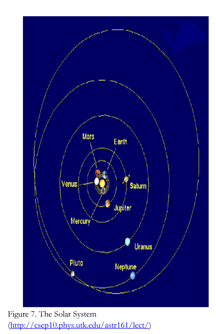
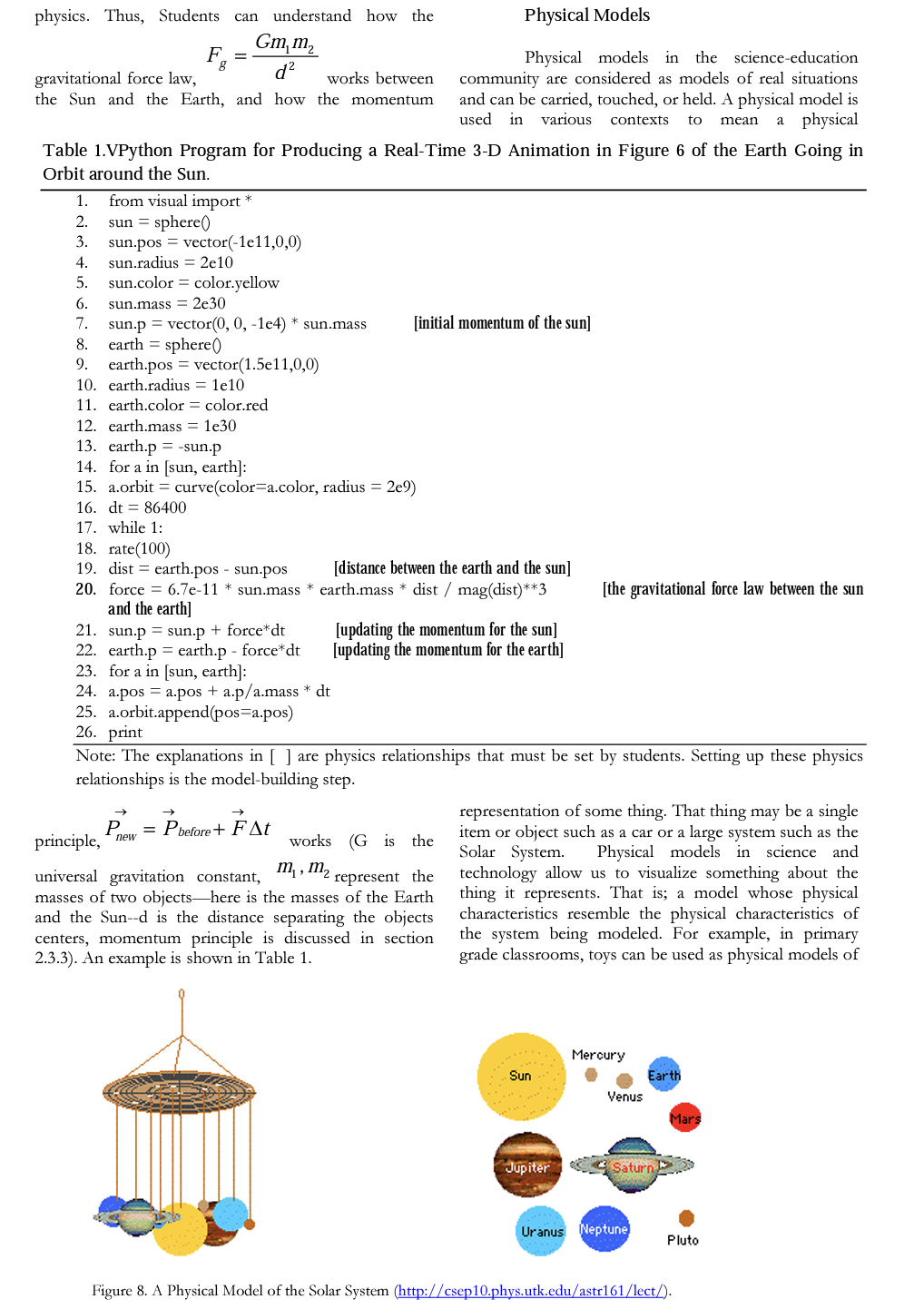
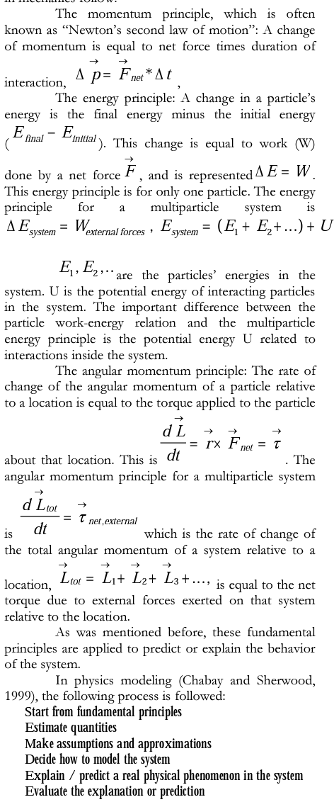
real-world counterparts. Toys model some of the functions of the real-world objects such as cars (Rogers, 2000). As mentioned above, a physical model of the Solar System (Figure 7) can be made by representing the Sun and the nine planets that orbit it. Several different ways can be used to do this. One uses cardboard colored circles of construction paper and string to make a physical model of our solar system as shown in Figure 8 (http://csepl0.phys.utk.edu/astrl61/lect/).
The Figure 7 of the Solar system shows the relative sizes of planets, but not actually to scale and shows their places in the system such as Mercury in the first orbit, Venus in the second orbit, Earth in the third orbit, Mars in the forth orbit, Jupiter in the fifth orbit, etc. Also, it shows that all of the planets orbit the Sun.
In Figure 8, since the range in size of the Sun and the planets is far too large to represent accurately, the Sun is showed as the bigjest. Jupiter, Saturn, Uranus, and Neptune are a bit smaller than the Sun. The remainder of the planets is much smaller. That Saturn has rings should be considered as well. So, students can see relative sizes of planets and can see that the nine planets orbit the sun. In addition, they can see that Mercury goes in the inner orbit, Venus goes in the second orbit, etc. After that, students can see the nine planets orbit the Sun.
Physics Models
Modeling means something different to physicists. A physics model in the physics-education community is considered as a simplified and idealized physical system, phenomenon, or idealization. Also, a mathematical model can be a component of a physics model. For instance, in the physics model of a gas, the gas is considered as many small balls which interact with each other by means of perfectly elastic collisions. Because the gas is ideal, we can apply the mathematical rules of classical mechanics. According to Greca & Moreira (2001), the physics models determine, for instance, the simplifications, the connections, and the necessary constraints. As an example one can think of a point particle model of a system in classical mechanics. A simple pendulum is another example of a physics model because it is idealized and consists of a mass particle on a massless string of invariant length moving in the homogenous gravitational field of the Earth in the absence of drag due to air (Czudkova & Musilova, 2000).
In terms of physics models, students do not use models which are already created. They apply the fundamental principles and create their own models. Modeling involves making a simplified, idealized physics model of a messy real-world situation by means of approximations. Then, the results or predictions of the model are compared with the actual system. The final stage is to refine the model to obtain better agreement, if needed. Sometimes it may not be needed to modify the model to get more exact agreement with the real- world phenomena. Even though the agreement may be excellent, it will never be exact since there are always some influences in the environment that we cannot consider while we are building the models. For instance, while a rock is falling, the gravitational pull of the earth and air resistance are the main influences. However, there are also other effects such as humidity, wind and weather, Earth’s rotation, even other planets (Chabay & Sherwood, 1999).
Building a physics model always starts from some fundamental principles. The three principles used in mechanics follow:
In summary, physics modeling is analysis of complex physical systems by means of making conscious approximations, simplifications, and
idealizations. When students make approximations or simplifications, they should be able to explain why they make them. For instance, in modeling a falling ball, in general, air resistance is neglected. So, there is no force contribution from air resistance. While students do neglect it, they should be able to have reasons for this. As an example of modeling, consider the calculation of the acceleration of a block is pulled to the right with a force F as shown in the following Figure 9.
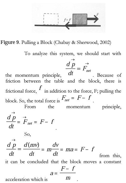
In these more traditional physics courses, students use constant acceleration to solve a problem instead of developing their own models. “Constant acceleration” is a mathematical model which is already defined for them. They do not bother to think about air resistance or friction. They are taught to select an equation to solve the problem. Moreover, even though students neglect friction or something in the system with respect to conditions, they do not do it consciously.
The following example shows how to make use of physics modeling to explain a real-world phenomenon, which can also be considered as a physics problem.
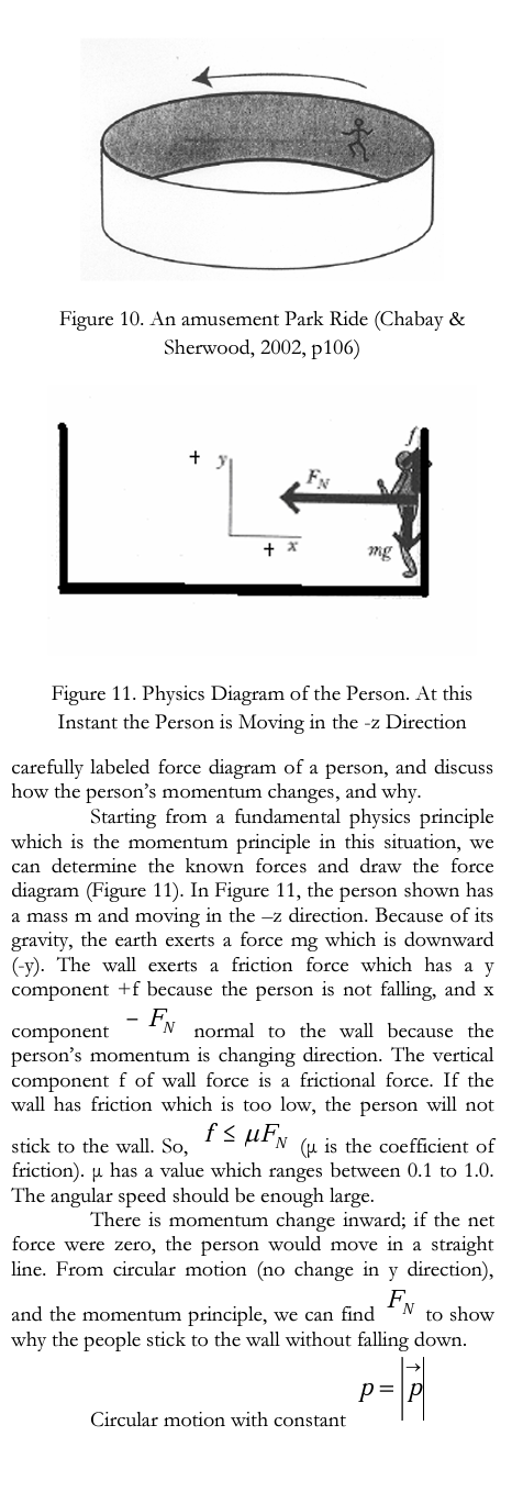
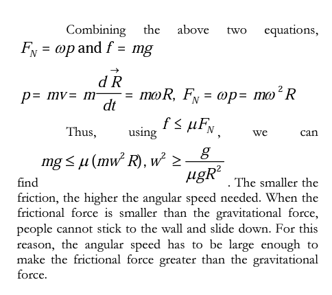
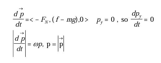
An amusement park ride (Chabay & Sherwood, 2002, pl06): There is an amusement park ride that some people love and others hate in which a group of people stand against the wall of a cylindrical room of radius R, as the room starts to rotate at higher and higher angular speed co (Figure 10). When a certain critical angular speed is reached, the floor drops away, leaving the people stuck against the whirling wall. Explain why the people stick to the wall without falling down. Include a carefully labeled force diagram of a person, and discuss how the person’s momentum changes, and why.
SUMMARY AND FINAL
CONSIDERATIONS
The emphasis of this paper lies on the discussion of different types of models and application of models and modeling with respect to the teaching and learning science particularly physics. These are mainly mental models; conceptual models, which are mathematical models, computer models, and physical models; and physics models.
The goal of this paper concerning different types of models in science education is to help teachers and students in order to learn how to use and choose models in their courses. Also, the most important aim is to make that students can be actively engaged in understanding and learning the physical world by constructing, using, or choosing models to describe, explain, predict, and to control physical phenomena (Wells et al., 1995). So, students do not need to memorize course materials or equations for their courses. They can obtain them by using models. From my experience with students who were taking an introductory physics course at Purdue University, students indicated that they can understand better concepts, the meaning of all equations, and how to obtain those equations in physics by using physics models. The following quotation explores students’ thoughts about physics models.
Student: ...there’s more to just physics than memorize this humongous block of equations the teacher says works. Uh, and plugging in the numbers and knowing how to put the equations together. We’re going back and- well we can- we’re really creating a model of this system and we can, you know, get rid of these factors because the gravitational pull is here is really not going to effect how me jumping off a chair is going to do anything. So what we can neglect even though there really is a force there it’s small enough that we don’t have to. Just kind of learning about physics in a very organized- and going back to elementary steps manner (Spring 2005).
As a result, models provide an application of the knowledge to real world situations-made to see how things apply in the real world instead of just looking at equations. In other words, helped students learn and understand physical phenomenon.
REFERENCES
- A Physical Model of the Solar System (n.d.). Retrieved June 15, 2005, from (http://csep10.phys.utk.edu/astr161/lect/)
- Buckley, В. C., Gobert, j. D., Kindfield, A. С. H., Horwitz, P., Tinker, R. F., Gedits, B.,Wilensky, U., et al. (2004). Model-based teaching and learning with BioLogica: What do they learn? How do they learn? How do we know? Journal of Science Education and Technology, 13, 23-41.
- Burghes, D. N. & Borrie, M. S. (1979). Mathematical modeling: A new approach to teaching applied mathematics [Electronic version]. Physics Education, 14, 82-86.
- Burghes, D. N. (1980). Teaching applications of mathematics: mathematical modeling in science and technology. Innovation and Developments, 365-376.
- Chabay, R. W. & Sherwood, B. A. (2002). Vol I: Matter and interactions: Modem mechanics. New York: John Wiley & Sons, Inc.
- Chabay, R. W. & Sherwood, B. A. (1999). Bringing atoms into first-year physics [Electronic version], American Journal of Physics, 67, 1045-1050.
- Czudkova, L. & Musilova, J. (2000). The pendulum: A stumbling block of secondary school mechanics. Physics Education, 35, 428-435.
- Driel, F. H. V. & Verloop, N. (1999). Teachers’ knowledge of models and modeling in science. [Electronic version]. International Journal of Science Education, 21, 1144-1153.
- Franco, C. & Colinvaux, D. (2000). Grasping mental models. In J. K. Gilbert & C. J. Boulter (Eds.), Developing models in science education (pp.93-118). Dordrecht, The Netherlands: Kluwer Academic Publishers.
- Gilbert, J. K., Boulter, C. J. & Elmer, R. (2000). Positioning models in science education and in design and Technology education. In J. K. Gilbert & C. J. Boulter (Eds.), Developing models in science education (pp.3-17). Dordrecht, The Netherlands: Kluwer Academic Publishers.
- Greca, I. M. & Moreira, M. A. (2002). Mental, physical, and mathematical models in the teaching and learning of physics [Electronic version]. Science Education, 1, 106- 121.
- Greca, I. M. & Moreire, M. A. (2000). Mental models, conceptual models, and modeling. [Electronic version]. International Journal of Science Education, 1,1-11.
- Hestenes, D. (1996, August). Modeling methodology for physics teachers. Proceedings of the International Conference on Undergraduate Physics Education, College Park, MA.
- Hestenes, D. (1987). Toward a modeling theory of physics instruction. American Journal of Physics, 55, 440- 454.
- Hodgson, S. M, Rojano, T., Sutherland, R. & Ursini, S. (1999). Mathematical modeling: The interaction of culture and practice [Electronic version]. Educational Studies in Mathematics, 39,167-183.
- Holland, D. (1988). A software laboratory. Dynamical modeling and the cellularmodeling system. SSR, 407- 416.
- Jimoyiannis, A. & Komis, V. (2001). Computer simulations in physics teaching and learning: A case study on students’ understanding of trajectory motion [Electronic version]. Computers & Education, 36, 183-204.
- Norman, D. A. (1983). Some observations on mental models. In D. Gentner & A. L. Stevens (Eds.), Mental models (pp. 7-14).Hillsdale, New Jersey: Lawrence Edbaum Associates, Inc.
- Scherer, D., Dubois, P., & Sherwood, B. (2000). VPython: 3D interactive scientific graphics for students. Computing in Science and Engineering, 82-88.
- The solar system, (n.d.). Retrieved June 15, 2005, from http: / / cseplO.phys.utk.edu/ astrlöl/lect.
- Tregidgo, D. & Ratcliffe, M. (2000). The use of modeling for improving pupils’ learning about cells. School Science Review, 81, 53-59.
- Vosniadou, S. & Brewer, W. F. (1992). Mental models of the earth: A study of conceptual change in childhood. Cognitive Psychology, 24, 535-585.
- Vosniadou, S. (1994). In mapping the mind. In S. A. Gelman & L. A. Hirschfeld (Eds.), Universal and culturespecific properties of children’s mental models of the earth. Cambridge: Cambridge University Press.
- Wells, M, Hestenes, D., & Swackhamer, G. (1995). A modeling method for high school physics instruction [Electronic version]. American Journal of Physics, 63, 606-619.
Related Articles
Ivan Ivanchei
Alves P.F.
Lohmander M.K.
Samuelsson I.P.
Dr Michael Skoumios
Chantal Pouliot
Barbara Bader
Geneviève Therriault